A variety of interesting LightLike simulation studies can be performed without explicitly modeling any relative motion of the subsystems. This type of simulation has the following structure:
(1) Using one value of a random number seed, define one realization of a sequence of phase screens between source(s) and sensor(s). The seed would be entered, for example, in the AtmoPath module.
(2) Propagate the optical beam(s) to obtain one statistical realization of the field(s) at all sensors. This constitutes one "run", as recorded in the .h5 file.
(3) Using the looping capability in the Run Set Editor, change the random number seed and generate a new (independent) realization of the sequence of phase screens, and propagate the optical beam(s) once more.
(4) Repeat N times.
This type of simulation produces N statistically independent sample results from each sensor, and is useful for certain types of statistical studies of turbulence effects.
Side remark: In the above type of statistical study, the simulation Stop Time parameter should be set so that only one sensor exposure is recorded for any run, given the exposureInterval of the sensor. Otherwise, one "run" in the .h5 file will contain identical repetitions of the sensor results for a given screen set realization. The duplicate results would all be correct, but execution time and storage would be wasted.
Although the type of statistical study described above is important, a more general scenario involves simulating the relative transverse motion of subsystems, while sampling the optical beams at specified rates. The key modeling assumption is that the phase screens, which are generated at the beginning of a run, move relative to sources and sensors according to the frozen-flow concept. Any study that involves rates of temporal evolution, such as calculation of the effectiveness of turbulence compensation and adaptive optics, is of this type. In such studies, the LightLike system must contain one or more subsystems that define relative motion between various parts of the system. In this case, one "run" of the simulation, as defined by the recorded .h5 data, consists of sensor results for a designated number of time steps. The number of time steps is determined by sampling rates defined in sensor subsystems together with the simulation Stop Time. The entire simulation may consist of only one "run" that lasts the designated time. Alternatively, using the loop capability in the Run Set Editor, the entire simulation may consist of several statistically independent runs of the same temporal length, that differ only in the seed used to generate the phase screens set. For any given run, a given phase screen set is generated, and subsequently the appropriate translations cause the optical beams to interact with different portions of the screens as the subsystem positions evolve in time.
As discussed in the preceding sections on sensor timing, LightLike always makes use of the concept of propagation delay (finite light speed) when computing the optical field that impinges on a sensor at any time t. This has a number of consequences when we construct LightLike systems and define parameters that specify transverse motion. The following sections discuss in detail how transverse motion is specified in LightLike, and how one handles the related effects of propagation delay.
Methods of implementing relative transverse motion
LightLike provides the following procedures for specifying the relative motion of sources, sensors and turbulent medium:
(1) The LightLike module TransverseVelocity specifies a transverse offset between modules located on the negative-z and positive-z sides (incoming and outgoing sides) of TransverseVelocity. The transverse offset may be static or time-varying. TransverseVelocity blocks can be used to model uniformly moving platforms and/or targets, and/or a uniform atmospheric wind. Some examples and details of TransverseVelocity and Slew usage are given below.
(2) Frequently, it is also necessary to use a Slew module in conjunction with TransverseVelocity, in order to keep beam(s) centered on sensor entrance pupils, and to keep focal spots at a fixed field angle on camera focal planes. This corresponds physically to tilting a transmitter or receiver system in order to stay pointed at the nominal position of a target or source. However, the need for Slew depends on the type of source and sensor being used.
(3) When a TransverseVelocity block is present, LightLike internally computes the implied relative displacement of each phase screen and any propagating beams. But in addition, extra transverse velocities may be explicitly assigned to the individual phase screens by using input arguments in the AcsAtmSpec function. AcsAtmSpec is typically used in a setting expression in AtmoPath or similar modules. The velocities entered in AcsAtmSpec are usually reserved to represent a true atmospheric wind which varies along the propagation path. As noted in paragraph (1), a uniform atmospheric wind can be modeled using just the TransverseVelocity modules.
The combination of procedures (1), (2) and (3) allows the LightLike user to input rather general motion specifications for platform, target and true atmospheric wind in a natural way. By "natural", we mean that target and platform velocities would be specified in TransverseVelocity modules, and true atmospheric wind velocities would be entered as arguments of AcsAtmSpec in AtmoPath or analogous modules. As noted above, in the special case where the true atmospheric wind is uniform, it may be easier to combine the true wind with the platform and target velocities in TransverseVelocity blocks. Examples below will illustrate this. Another alternative, if the user wishes to exercise it, is to manually calculate the net pseudo-wind velocity that characterizes the motion of each phase screen relative to the beam(s). Algebraic expressions for these velocities could then be applied to the screens in AcsAtmSpec, and one could dispense with the TransverseVelocity module completely. This is a common procedure in wave-optics simulation, but in the LightLike world the usual practice is to use the combination of methods (1), (2) and (3) outlined above.
The principal restriction on LightLike motion specifications is uniformity, i.e., constant linear and angular velocities. This is really no defect since, over the time scales that are practical for most wave-optics simulation, practical platform and target systems will not appreciably change velocity. Jitters induced by atmospheric turbulence and by platform or target base jitter are not contrained by the uniformity assumptions under discussion here.
Use of the TransverseVelocity module
As we see from the picture at right, the TransverseVelocity module takes two pairs of parameter specifications, named (x0, y0) and (vx, vy). The pair (x0, y0) defines an initial offset at t=0. This offset is the displacement of the local (x,y) coordinate origin on the negative-z side of TransverseVelocity with respect to the (x,y) origin on the positive-z side of the module. The pair (vx, vy) defines the velocity (signed) of the (x,y) coordinate origin on the negative-z side of the module with respect to the (x,y) origin on the positive-z side of the module. As we will see below, a LightLike system often contains two TransverseVelocity modules to model the motion of Platform and Target groups relative to the turbulent medium and to each other. In general, there is no limitation on the number TransverseVelocity blocks that may be inserted to produce offsets among the blocks of a system.
In the special case (vx, vy) = (0,0), TransverseVelocity can be used to define a static offset between the modules on the negative and positive sides of the TransverseVelocity block. If (vx,vy) is not (0,0), then a time-varying offset between the local origins on either side of TransverseVelocity is generated. The offset of the negative-z relative to the positive-z side will be
xoff = x0 + vx · t , yoff = y0 + vy · t ,
where t is the simulation virtual time.
As mentioned in the section on spatial coordinate systems, the fields and mathematical support regions of sources, sensors, apertures, apodizers, and other such modules are defined with respect to each module's local (x,y) coordinate origin. The origins of all the local (x,y) coordinate systems are then related by the following rule: the local (x,y) origin of any module "lines up" with the origin of its neighboring module, unless the modules are separated by a TransverseVelocity block that generates an offset (static or dynamic). In a few cases, e.g., PointSource, a module may itself provide static decentering parameters with respect to the local module origin, but in most cases transverse offsets must be achieved using a TransverseVelocity block placed between modules. When a LightLike system contains more than one TransverseVelocity block, the offsets add vectorially.
The internal workings of LightLike do not define any global (x,y) origin. However, the user will probably find it clearest to mentally set up the problem in terms of a global coordinate system, usually fixed with respect to the earth. Then, the expressions for the relative velocities and positions required by the LightLike modules can be derived fairly simply. As an example, consider the following motion specifications which form the basis for the LightLike examples to be diagrammed in the remainder of this section.
Example motion specification:
(1) A global coordinate system fixed with respect to the earth.
(2) A global z axis (nominal propagation direction) along a specified elevation angle.
(3) A uniform horizontal atmospheric wind, with velocity v = (vx, vy) = (0, wy) with respect to the global coordinate system. (Bold symbols in this section denote vectors). Remember that x and y axes can be any two orthogonal directions transverse to z. By defining v = (0, wy), we have associated y with the horizontal direction that is perpendicular to our propagation direction z.
(4) A source with velocity v = (vx, vy) = (0, 0) with respect to the global coordinate system.
(5) A receiver subsystem whose velocity v = (vx, vy) = (vRx, vRy) with respect to the global coordinate system.
In the following System Editor screenshot, we begin to build a LightLike system that incorporates the above motion specifications. We will build the system incrementally, and we will consider some variations in behavior related to the type of source we use. We begin by using a PointSource, a pair of TransverseVelocity blocks sandwiched around an AtmoPath propagator block, and a receiver group consisting of a Telescope and Camera. (Side remark: Alhough not essential for present purposes, the user may wish to better understand the functions of Telescope and Camera in the LightLike system. Briefly, LightLike's Telescope is simply a combination of a Focus and an Aperture. The focus is used to force Camera's focal plane to be conjugate to something other than infinity. See "Using the Camera module" for details).
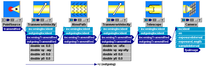
The block i/o connections designate the wave emanating from the source to be "outgoing". Consequently, in LightLike terminology, this source is at the "platform" end (negative-z end) of the propagation path, while the receiver group is at the "target" end (positive-z end). As defined earlier, the platform-target orientation is significant when defining the signs of parameters in TransverseVelocity. Now, given the global motion specifications (1)-(5), and the direction conventions just reviewed, we define the input parameters of the TransverseVelocity modules in terms of the following relative velocities:
(a) Velocity of PointSource with respect to AtmoPath (i.e., the air medium): v01 = (0, -wy)
(b) Velocity of AtmoPath (the air medium) with respect to Telescope (and to all other receiver modules): v02 = (-vRx, +wy - vRy).
The System Editor diagram shows the components of v01 and v02 inserted into the (vx, vy) value fields of the TransverseVelocity parameter lists. Users should study this example carefully and understand how the v01 andv02 relative velocities are consistent with the definitions stated earlier for the TransverseVelocity (vx, vy) parameters. A user who understands the above basic example will be able to generate any elaborations, such as adding a non-zero velocity for the source.
In the preceding example, the t=0 offsets in both TransverseVelocity blocks have been set to zero: (x0, y0)=(0,0) in each block. That is, at t=0, the local z axes of all modules are exactly colinear. These specifications were not explicitly defined in the original global specs (1)-(5). Depending on problem details, the user may wish to key the initial offsets (x0,y0) to the propagation delay time (prop distance)/c. For example, one may wish the detector center to be at a specific transverse location at the time the first light (emitted at t=0) reaches the detector: in that case, the values of the (x0,y0) parameters must be expressed in terms of the transverse speed and the delay time.
Uniform atmospheric wind:
In the above example, note a key point regarding the uniform atmospheric wind specification. It was possible to model the uniform wind, plus the effects of platform and target motion, all using the TransverseVelocity blocks. That is, to model uniform atmospheric wind, it is not necessary to enter any wind specifications in the AcsAtmSpec function (recall the overview of transverse motion methods). The velocities entered in AcsAtmSpec are usually reserved to represent a true atmospheric wind which varies along the propagation path, although the preferred modeling practice is up to the user.
Use of the Slew module
Consider again the LightLike system defined in the preceding System Editor picture. The drawing at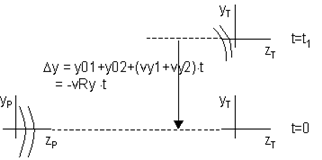 right shows the local coordinate axes of the platform (P) and the target (T) at two time instants. Because the parameters (x0,y0) = (0,0) in both TransverseVelocity blocks, the local z axes are colinear at t=0. However, at later times, the telescope/camera's z axes get progressively further displaced from the source's z-axis. The drawing at right shows the situation in the y-z plane. Now, the PointSource module has a special property relative to any other source type in LightLike. In particular, regardless of the transverse offset between PointSource and a sensor, the LightLike machinery will always compute a propagated field whose support is centered at the origin of the sensor's effective pupil plane. To put it simply, PointSource operates in such a fashion that it always "points" at a sensor, regardless of the sensor local origin's transverse offset. This behavior is not obligatory for numerical calculation, but it is certainly consistent with the typical interpretation of "point source".
Slewing the transmitter:
By way of contrast, suppose that we replace PointSource in the above system by GaussianCwLaser (or UniformWave, or in general any "extended" source module available in LightLike). In that case, the phase in the exit plane of the source gives the source wave a uniquely defined direction, which is usually nominally parallel to the local z axis of the source module. Since such a beam has a finite extent, within diffraction, it is then possible that the beam can miss the sensor if the transverse displacement is large enough. If that effect is what the user is trying to model, then nothing further needs to be done. However, the more usual physical situation is that the transmitter is slewing at a fixed angular rate, in order to track the target. That is, within the perturbations caused by turbulence, we want to keep the transmitted beam pointed so that its centerline moves with the target. The modified LightLike system in the following picture shows how this is done. We have modified the previous system by replacing PointSource with GaussianCwLaser, and by adding a Slew module immediately after the source:
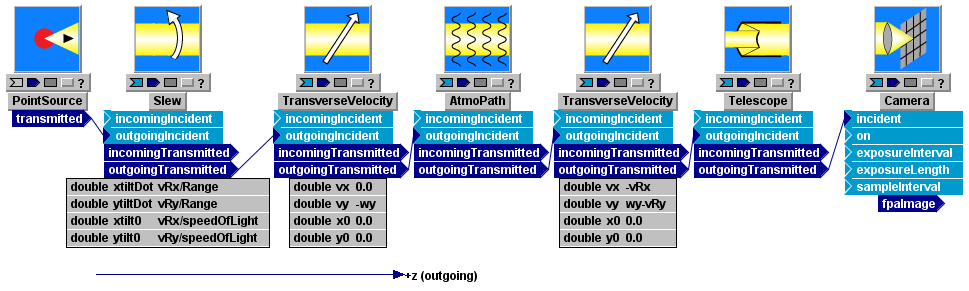
The velocity parameters that were already specified in the TransverseVelocity blocks now dictate the angular rates and the initial (t=0) offsets that we must enter in the Slew block parameters. The velocity of the targetrelative to the transmitter is vrel = (vRx-0, vRy-0), independent of the uniform wind wy. Therefore, the Slew block will cause the transmitted beam to (nominally) track the target if we specify the following angular rates:
(xtiltDot, ytiltDot) = (vRx / Range, vRy / Range) rad/s,
where Range is the propagation range. (The variable Range is also a parameter entry in the AtmoPath block in the above system, but those parameters are not pulled for viewing in the present pictures). This angular rate specification keeps the beam slewing at the same rate as the target.
Additionally, we also wish to center the beam on target (strictly speaking, on the local coordinate origin of the target's entrance pupil). Recall that in the two TransverseVelocity blocks, we specified both t=0 offsets (x0,y0)=(0,0). This means that the local z axes of source and receiver pupil are colinear at t=0. Consequently, to make the emitted beam's centerline strike the center of the receiver pupil, the Slew must allow for propagation delay by pointing ahead of the present receiver position by the following angles:
(xtilt0, ytilt0) = (vRx / speedOfLight, vRy / speedOfLight) rad.
Note that the Slew block parameters (xtilt0, ytilt0) are not the lead-ahead angles per se, but rather are defined as the Slew angles at t=0. Because we had set (x0,y0)=(0,0) in both TransverseVelocity blocks, we have the simple situation that the initial offset slew angles (xtilt0, ytilt0) are numerically equal to the lead-ahead angles.
Slewing the receiver, for different types of LightLike sensor:
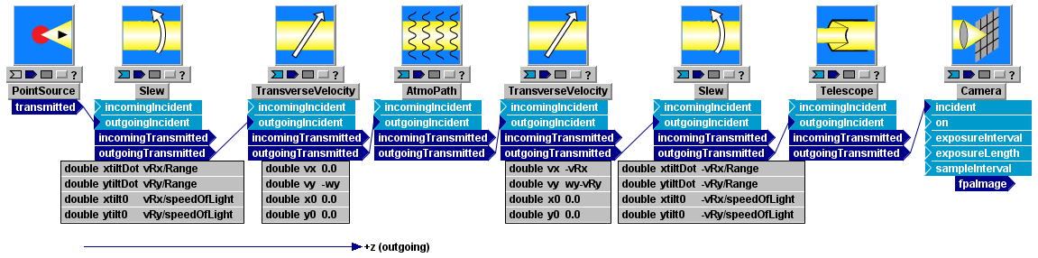
The modified system that we just created keeps the GaussianCwLaser beam pointed at the target, and centered on the target's entrance pupil. However, the Camera subsystem still has its local z axis parallel (though offset) to the local z axis of the source laser. Therefore, the focal-plane intensity spot reported by Camera will march progressively more and more off-axis as time proceeds, and may go entirely off the focal-plane sensor, depending on the specified size of that sensor. If the modeling intent is to keep the Camera z-axis pointed at the source as the motion proceeds, then another Slew module must be added just in front of the Telescope subsystem. The angular rate parameters of that Slew module would need to be
(xtiltDot, ytiltDot) = (-vRx / Range, -vRy / Range) rad/s.
With this additional Slew module at the receiver, the Camera focal plane spot will stay centered (within atmospheric turbulence) on the Camera sensor plane local origin. The final system, with two Slew blocks, is shown in the following figure:
In addition to Camera, the other two principal LightLike sensor modules are TargetBoard and SimpleFieldSensor. The user should understand the effect of receiver slewing in each case. If the receiver in the above system consisted of a TargetBoard, instead of the Telescope-Camera combination, then slewing the receiver would have no effect. In the case of TargetBoard, the sensor just measures irradiance of the propagating beam in the plane of the target-board, and that is essentially unaffected by the range of offset angles that one can treat in LightLike. We expand on this point in the following paragraph.
If the receiver consisted of a SimpleFieldSensor, instead of the Telescope-Camera combination, then slewing the receiver would have no effect on the irradiance, but it would have an effect on the sensor's output phase. In the case of SimpleFieldSensor, the sensor outputs the complex field of the propagating beam, in the plane of the sensor. The irradiance formed from the complex field output should behave just like the output of TargetBoard, hence is unaffected by the receiver slew. However, the phase computed from the output of SimpleFieldSensor issensitive to typical offset angles modeled in LightLike. As an example, suppose the local origin of the target plane is offset by 1 mrad (a very large angle for most LightLike purposes) from the transmitter local origin. Suppose further that the optical wavelength is 1 mm, the sensor transverse span is 10 cm, and the beam phase is roughly planar and perpendicular to the line from source to sensor. Then, if the sensor were precisely parallel to the x-y plane, it should see a phase difference of (1E-4m/1 mm)=100 waves across the 10 cm of sensor span. On the other hand, if a compensating Slew of (-1) mrad were inserted just prior to the sensor, then the sensor would report zero waves of phase difference across the sensor span (in the plane-wave approximation). In contrast to the phase dependence, the irradiance projection factor is for all practical purposes 1.0 with or without the receiver slew.
(Side remark: Actually, the irradiance projection factor is completely ignored by LightLike. This is really not a defect, because other modeling limitations in LightLike would be exceeded long before the irradiance projection became measurable).
We introduced the functions of the Slew module only after switching from PointSource in the original system example to GaussianCwLaser in the second system example. We chose that order of presentation because we wanted to treat transmitter slewing before receiver slewing. Near the beginning of the slew section, we explained that PointSource is coded in such a way that slewing the transmitter is not necessary. But now, based on the above sequence of examples, the reader can probably see that receiver slewing is still necessary for PointSource, if we use the Camera sensor and we wish to keep the image point centered on Camera's focalplane.
Slew and Tilt:
In terms of the internal workings of LightLike, the Slew subsystem is simply a (uniformly) time-varying Tilt subsystem. To understand modeling limitations, the LightLike user should have some basic understanding of how tilt is implemented in LightLike: this is discussed in the section "How tilt is modeled".
TransverseVelocity, Slew and Tilt for counterpropagating beams:
The above example has only an outgoing optical wave, but more complicated systems can simultaneously have outgoing and incoming waves. Notice that the TransverseVelocity and Slew (or more basically, Tilt) modules have input/output connections for both directions of waves. Suppose that, after setting up the velocity and slew parameters in the above system based on consideration of the outgoing wave, we now decide to add an incoming wave, by adding a source at the original target end, and a sensor at the platform end. The LightLike sign conventions are consistent in the sense that the existing transverse velocity and slew specifications are still appopriate: we need not go through that setup procedure twice.
Slew tilts the wave, not the sensor:
In order to thoroughly understand and apply the LightLike rules and conventions regarding slew and tilt, it will be helpful for the user to understand the following. In the internal workings of LightLike, the receiver-end slew added to the above system acts on the propagating wave, not on the sensor per se. While it is acceptable to think of the slew as causing the central line of sight of the sensor to rotate at the rate (xtiltDot, ytiltDot), what is actually happening at the code level is that the tilt parameter associated with the passing wave is adjusted by the specified angle or angular rate. In this connection, we must remember LightLike's sign convention for tilt, which also governs the Slew module signs.
An apparent paradox related to transverse motion and wavefront tilt
When a simulation involves relative motion, we have the possibility of analyzing the problem from the point of view of different reference frames. This can lead to some apparent paradoxes involving the numerical value of wavefront tilt measured by a sensor. As we have seen in the preceding sections on sensor timing and transverse motion, LightLike combines the following two concepts: (a) propagation delay (finite light speed) is always applied when computing the optical field that impinges on a sensor at any time t; (b) coordinate and velocity transformations between reference frames are assumed to obey the Galilean model. Additionally, the propagation delay is approximated by (L/c), where L is the z-separation of source and sensor local origins. Reasoning based on the preceding concepts, exemplified in the preceding discussions of transverse motion and slew, is generally adequate in the regime where transverse velocities of sources, targets and medium are small compared to the speed of light, c, and where the transverse offsets are small angles.
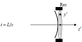
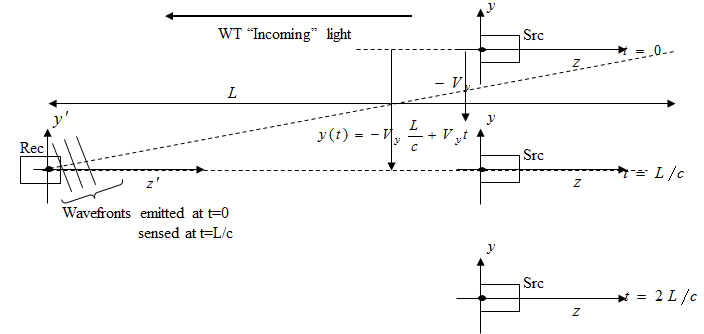
Despite the general adequacy of the {delay + Galilean transformations} model, it is possible to generate an apparent paradox with this reasoning, regarding an offset in the observed value of wavefront tilt. We mention the issue in this Guide because several LightLike users, both external and internal to TimeLike Systems, have been puzzled by it. Consider the following simple propagation problem: (a) a receiver detects waves emitted by a point source, in the absence of atmospheric turbulence; (b) there is relative transverse motion with uniform velocity, and the transverse offset between local coordinate origins is 0 (local z axes colinear) at time t = L/c. First, consider the situation in the rest frame of the receiver. The following sketch shows the transmitter position at several instants, and shows the "first light" wavefront striking the receiver pupil (assuming emission begins at LightLike's usual t=0):
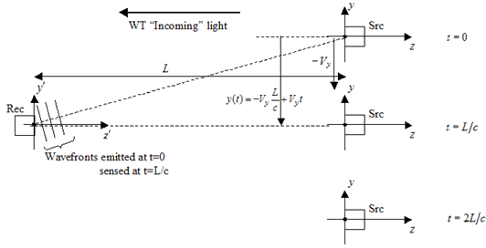
From this sketch, we conclude that tilt of the received wavefront at t=L/c is ytilt' = -Vy/c (the minus sign is consistent with the LightLike tilt sign conventions). If the corresponding LightLike system is constructed with PointSource, AtmoPath, and SimpleFieldSensor or Camera blocks, the user can confirm that this is the tilt answer reported by LightLike. In fact, the reasoning related to the delay time from the point of view of the sensor that led to the above sketch and conclusion is exactly what LightLike does internally.
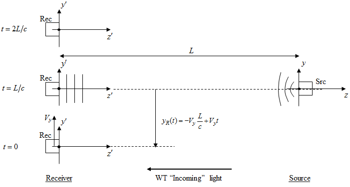
Now the paradox arises as follows. Let us consider the situation in the rest frame of the source. The following sketch shows the receiver position at several instants. From this point of view, the
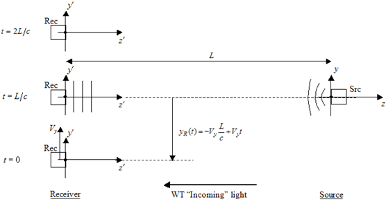
wavefronts anywhere along the z axis are perpendicular to z, so at the instant t=L/c it appears that the receiver should report ytilt = 0. This clearly contradicts the result inferred from the first approach. In the detailed discussion that follows, we discuss this paradox at greater length, from several other points of view, and we argue that the first result (the LightLike result) is the correct one.
Detailed Discussion of some aspects of wavefront tilt and relative motion
There is an aspect of the wavefront tilt reported by LightLike when the receiver is moving relative to the source. Analysis of the problem from the point of view of different reference frames seems (at first) to have some paradoxical features. The issue is connected with concepts and methods of special relativity, but we can discuss and resolve the issue without the full relativity analysis machinery.
In rest frame of source, let:
•Source emit initially collimated beam with 0 tilt, or on-axis spherical wave
•Receiver move transverse to propagation direction, with offsets and timing as shown
Provisional conclusion: analysis 1 implies that measured tilt (avg) of wavefront reported by sensor at t = L/c should be q’y = 0.
Before inquiring what tilt LightLike reports, let’s do another thought experiment (analysis 2). Continue to visualize in rest frame of source.
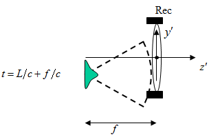
1.Explicitly consider time (f /c) required for wavefront to propagate from receiver pupil to image plane.
2.Image plane centroid, y’c , satisfies
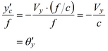
3.The time at which result (2) is valid is slightly > (L /c), but if f <<L, this is for all practical purposes = (L /c). Note that angle is independent of f.
4.Typical (Vy /c) values: (10m/s) / 3E8m/s = 0.033 urad
(1000m/s) / 3E8m/s = 3.3 urad
5.Provisional conclusion: “tilt” prediction from analysis 2 contradicts analysis 1. Suggests a non-unique connection between wavefront tilt and reported centroid.
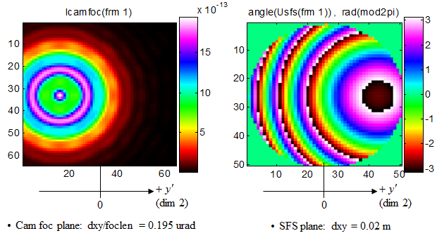
•Images from the two LightLike sensors, at t = L/c (first data frames recorded by the runset timing setup). (Note that LightLike expLen =1E-12s, negligible)
•Lightlike’s tilt answer (from both sensors): q’y = - 3.3 urad = -(Vy /c) LightLike gives the “analysis 2” answer.
•NOW, TWO QUESTIONS:
(A) Is the LightLike answer right or wrong?
(B) What logic did LightLike use? Note that LightLike got the “analysis 2” answer, but it definitely did not use that logic ...
In rest frame of receiver, we have the picture below
•Analysis concept: at t=L/c, receiver senses light emitted by source at earlier (t=0) time
•This light presumably has the tilt indicated at the receiver block diagram
•Provisional conclusion: analysis 3 implies that measured tilt (avg) of wavefront reported by sensor at t = L/c should be q’y = -(Vy /c).
•Analysis 3 conclusion is same as analysis 2 conclusion, but disagrees with analysis 1.
•Concept 3 is essentially the logic built into LightLike: LightLike's transverse motion manipulations are based on visualizing the problem in the rest frame of the receiver.
•Final question: is analysis 3 correct? After all, analysis 1 looks pretty convincing to some people.
In the Analyses 1 and 2: we said those pictures were drawn from the point of view of the source, but really it’s a sort of God’s eye view of the situation.
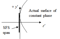
Formal analytical approach: write a formula that expresses the surface of constant phase in one reference system, and perform t-dependent coordinate transformation to obtain formula for surface in other system
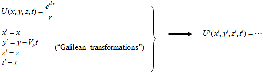
This approach yields same answer as analyses 2 and 3 (the LightLike answer)
Another picture frequently used that is equivalent to the formal coord transformation idea is to apply vector velocity addition to a point on the wavefront:
![]()
Special Relativity works the problem from the point of view of formal coord transformations, but using the Fitzgerald-Lorentz transformations.
Suggested homework:
•WT plane wave case (slew complication)
•Work out the formal Galilean coord coordinate transformation method
Transverse and longitudinal motion
All the commentary in this section applied to transverse motion. Issues relating to longitudinal motion are of a different character, and are discussed in a separate section.