Atmospheric turbulence models and the specification of turbulence phase-screen strengths and positions is discussed in another section. However, the desired size of the phase screens is more closely related to transverse motion, so we discuss that subject now.
The specification of the turbulence phase screen mesh parameters (dimension and spacing) is a separate step from, though logically related to, the propagation mesh specification. Desired screen mesh parameters are linked to the propagation mesh as well as to the transverse displacement of transmitter, receiver and air mass during the simulation time span. The screen mesh parameters are specified via parameters in one of the propagator modules such as AtmoPath or GeneralAtmosphere. These two modules are shown below, with their i/o and parameter lists pulled down.
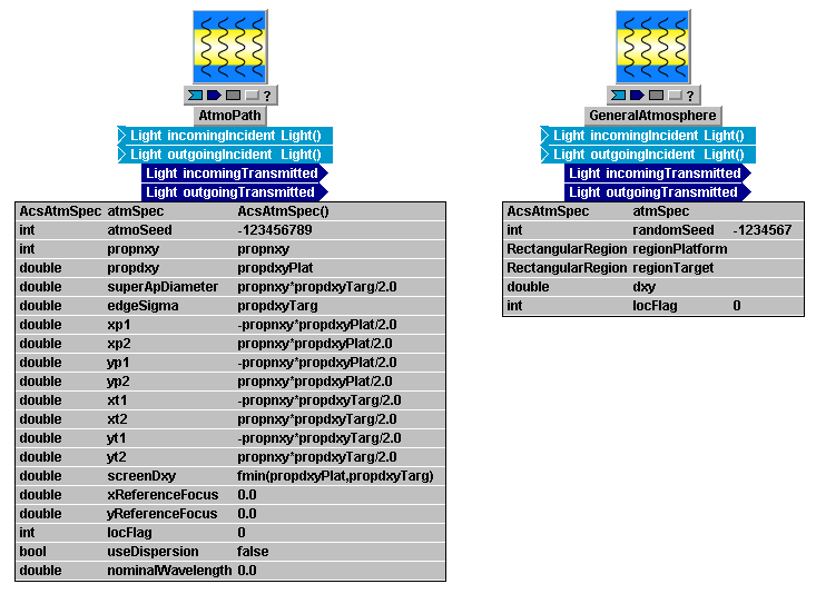
The concepts by which the screen meshes are specified in the various propagator modules are identical, but the parameter name notation and grouping differs slightly from one module to the next. Once the user understands the concepts, the naming variations should not cause any confusion. We will explain the key ideas in terms of the AtmoPath nomenclature. The relevant parameters in AtmoPath (see above figure) are the two groups {xp1, xp2, yp1, yp2} and {xt1, xt2, yt1, yt2}, plus the parameter screenDxy. The index numbers "1" and "2" should be understood as "min" and "max": 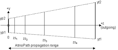 thus, the coordinates {xp1, xp2, yp1, yp2} define a rectangular region at the platform (p) side of AtmoPath, while the coordinates {xt1, xt2, yt1, yt2} define a rectangular region at the target (t) side of AtmoPath. The sketch at right illustrates the y dimension. (Note that the parameter values entered in the above AtmoPath diagram (third column in the parameter list) are merely the default values that are presented when one initially pastes AtmoPath into a user system.)
Once the user specifies values for the p-side and t-side rectangular regions, LightLike conceptually connects the endpoints by straight lines (dashed lines in the sketch), forming in two dimensions a rectangular frustrum. Finally, at the designated z coordinates of the phase screens (zsk in the sketch), LightLike creates phase screens that span the interior of the frustrum (as indicated one-dimensionally in the sketch). The rectangular frustrum algorithm is a general method for more or less optimizing the required sizes of the successive phase screens. In sum, by specifying rectangular x-y regions at the platform and target ends of the propagator module, the user implicitly specifies the size of all phase screens that will be used in that propagator module.
How large should the p-side and t-side rectangular regions be? The rectangles at the two ends must be at least as large as the propagation meshes used, and frequently should be larger, for two reasons. First, as the transverse positions of platform, target, and air mass evolve (assuming there is motion), the optical beams sample different portions of the phase screens. Ideally, the size of the p-side and t-side rectangular regions would be chosen so that at a given screen z the screen spans the entire width swept by the beam during the simulation. In practice this may not be feasible for long simulation times, so LightLike has the following provision. If the user-specified size of a screen is insufficient to span the area required by transverse motion, then LightLike automatically wraps the screen. Equivalently stated, whatever the user-specified size of the screen, LightLike will treat that screen as a periodic function whose period is the screen "size" specified by the user. As a result, any optical beam will always have some phase perturbation to sample, although that perturbation may repeat itself in time at a particular screen location. After we illustrate screen setup with a numerical example, we will discuss further how to avoid overall periodicity of the propagation results when we specify undersized rectangular regions.
There is also a second reason for making screen sizes bigger than the propagation mesh, which has nothing to do with motion. The issue here is a defect of the conditioned-white-noise method of generating 2D random functions. We discuss this second issue a bit more in a later section on screen details.
Numerical example of screen width specification based on motion
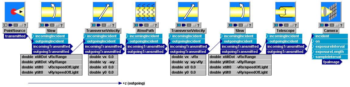
Let us consider a numerical example to illustrate the screen mesh specification. Consider again one of the LightLike systems used previously to illustrate transverse motion and slew. We repeat the system diagram here:
Suppose that:
(a) The transmitter-receiver z-separation is 100 km
(b) The platform velocity relative to earth is (0, 0)
(c) The receiver velocity relative to earth is (vRx, vRy) = (-20, +100)m/s
(d) The true-wind velocity relative to earth is (0, wy) = (0, +10 m/s)
(e) At t = 0, the receiver and transmitter local origins have zero transverse offset (x0 = 0 = y0 in both TransverseVelocity modules)
(f) We wish to simulate the receiver signals until t = 0.1s (= Tsim)
(g) The propagation mesh parameters propnxy (dimension) and propdxy (spacing) have been specified as discussed elsewhere, and for brevity we define ΔXYprop = propnxy * propdxy. (The x and y specifications of the propagation mesh are not required to be equal, but that is a common case). Suppose that ΔXYprop = 4 m has been specified.
We discussed in a previous section how the motion specifications (b)-(e) translate into the (vx,vy) and (x0,y0) value specifications that have been entered in the third columns of the two TransverseVelocity blocks. We are now in the process of determining the turbulence screen parameter values to be entered in AtmoPath. The key facts are:
(1) At the platform (z=0), the total displacement of the source modules relative to the atmosphere during the simulation time is (ΔXp, ΔYp) = (0, -wy*Tsim) = (0, -1.0) m.
(2) At the target end, the total displacement of the atmosphere relative to the target modules during the simulation time is (ΔXt, ΔYt) = (-vRx*Tsim, [wy-vRy]*Tsim) = (2.0, -9.0) m.
(3) The propagation mesh spans (ΔXYprop, ΔXYprop) = (4.0, 4.0) m. As explained elsewhere, because of LightLike's motion/wavefront-tilt procedures, we can think of the propagation mesh as having zero offset at all times despite the transverse motions.
Combining the maximum motion offsets with the size of the propagation mesh, i.e, the facts (1)-(3), we can fix phase screen sizes (regardless of their z locations) by specifying the following rectangular regions in AtmoPath:
(A) (xp1, xp2) = (-ΔXYprop/2, ΔXYprop/2) = (-2.0, 2.0) m
(yp1, yp2) = (-ΔXYprop/2, ΔXYprop/2 + | wy*Tsim |) = (-2.0, 3.0) m
(xt1, xt2) = (-ΔXYprop/2, ΔXYprop/2 + | vRx*Tsim |) = (-2.0, 4.0) m
(yt1, yt2) = (-ΔXYprop/2, ΔXYprop/2 + | wy-vRy |*Tsim) = (-2.0, 11.0) m.
For each pair of coordinates, we have added the absolute value of the relevant motion displacement to the upper bound of the zero-offset propagation mesh. Adding the magnitudes in this way is not the only viable approach, but it has one significant advantage. First, note that the screen periodicity discussed earlier means that (xp1, xp2) and the other pairs can be extended in either direction: it is not obligatory to extend the rectangular regions in the actual direction of motion. The principal advantage of using the absolute value method illustrated in (A) is that the algebraic combinations remain valid if one later changes the signs of the various velocities when executing parameter studies of the system behavior.
The alternative method, which might initially seem more straighforward, is illustrated by the following specification:
(B) (yp1, yp2) = (-ΔXYprop/2 - wy*Tsim, ΔXYprop/2)
If wy = +10 m/s, as in the original numerical specification, then the yp1 assignment in (B) explicitly accounts for the fact that a screen located at the platform would move towards +y by the amount DY = wy*Tsim, relative to the platform. But now a potential problem arises: suppose we defined yp1 algebraically as in (B), elevating the wy variable up to the runset where a numerical value is assigned. Suppose further that at some later time we are exploring parameter variations and we decide to assign a negative value to wy. Inspection of the (B) format shows that an error occurs unless we move the wy*Tsim contribution from the yp1 to the yp2 term. Similarly, in the term (wy-vRy) a net sign change can occur depending simply on whether wy is less or greater than vRy. As a general principle, it is inconvenient and error-prone to set up the system and runset so that changing the numerical value of a runset parameter requires us to make some compensating setting change lower down in the system hierarchy. For some system properties it may become too involved to maintain complete generality in this respect, but for the screen specifications the absolute value method (A) provides an easy solution.
In the specifications (A), we concluded with numerical values to give a sense of typical numbers. However, we would generally want to enter the algebraic setting expressions in AtmoPath, and to elevate variables like wy, vRy, etc. to the runset level: that makes it easy to perform parameter variations by just changing a few numbers in the runset. Detailed syntax rules and elevating procedures are discussed in TimeLike User's Manual; to conclude the present discussion we just point out one pertinent detail, namely that |x| must be entered in LightLike setting expressions as fabs(x).
Actual screen dimensions, computation time and memory requirements:
Thus far, the present section has concentrated on specifying the physical span of the turbulence phase screens. The final parameter required to specify the discrete screens is the mesh spacing, which in AtmoPath is called screenDxy. Typically, we set screenDxy equal to the propagation mesh spacing designated in some previous expressions as propdxy. Strict equality of screenDxy and propdxy is not obligatory, but is usually a reasonable choice.
Once the user has specified the spans (xp2 - xp1), ..., and the screenDxy, then the screen meshes are fully specified as far as the user is concerned. However, LightLike makes some further internal adjustments. At present, LightLike generates phase screens by starting with an uncorrelated random process in the frequency domain, spectrally conditioning that power spectrum, and then inverse transforming to obtain the space-domain screen realization. Since the Fast Fourier Transform (FFT) algorithm is used, LightLike adjusts the ratio (xp2 - xp1)/screenDxy upward to the nearest integer having a "nice" factorization for evaluating the FFT. Thus the screen dimension will actually be slightly bigger than implied by the precise user specifications.
Screens are only generated once per atmospheric realization, so that even very large screens may have small impact on simulation execution time. Propagation and motion evolution requires Fresnel propagation from source to first screen, then from screen to screen, then finally from last screen to sensor, for each time step of the simulation, but all with a single pre-computed set of screens (a single atmospheric realization). Therefore, even if the screens are much larger than the propagation mesh, it is often the case that execution time is dominated by the propagation calculations, and is only slightly affected by the initial generation of the screens. Of course the screens are used at each propagation step, but after the screens are generated by using the spectral conditioning method then each screen application during propagation is only a simple array multiplication.
On the other hand, required memory is strongly affected by the specified screen size. We cannot give specific limits on screen dimensions for various computer configurations, but we can give a few examples of dimensions that have been used with no ill effects. In the numerical example of screen specification given several paragraphs ago (at the (A) marker), the target-end rectangular region spanned 6x13 m in the XxY dimensions. Supposing that screenDxy=2 cm, that would imply (prior to the LightLike adjustment) a screen dimension at the target end of 300 x 650 points. This is a modest requirement in terms of modern personal computers. If we increased Tsim from 0.1s to 1.0 s, then the 6x13 m becomes 24x94 m, or a screen dimension of 1200x4700 points. This is still doable on a modern PC, but may be approaching the danger zone depending on the user's PC configuration.
Avoiding overall periodicity by various means
We noted above that LightLike's phase screens effectively scroll periodically if relative motion requires an optical propagation operation to sample a phase screen beyond its nominal edge. If all the phase screens repeated with the same frequency, then the optical results at a sensor would repeat exaclty with that frequency, making runs longer than that period useless. If there is a need to accumulate statistics over longer periods, several approaches can be considered.
The brute-force approach is to make the screens longer in the direction of motion, but as discussed above this has practical computer limits.
A simple approach would be to do repeated runs with different random number seeds for the screen set. The repeated runs cannot be joined end to end in post-processing because discontinuous jumps in results would occur at the joints. However, the method is perfectly satisfactory for accumulating certain types of statistics.
Another possibility is to note that overall periodicity can be mitigated significantly if the screens have different lengths or different transverse speeds. In that case, even though each screen is repeating periodically, the combined turbulence effect would only repeat over a much longer period, namely the least common multiple of the individual periods. Although some violation of nature is involved here, for most statistical purposes the approximation is probably quite good.