In the present section of the User Guide, we discuss certain important features of the core LightLike library components needed for wavefront sensing and correction. These core components are HartmannWfsDft, DeformableMirror, and BeamSteeringMirror.
The generation of some of the geometric input specifications and the reconstruction matrices required by HartmannWfsDft and DeformableMirror is a complex task. A separate Adaptive Optics Configuration Guide has been written to explain the extensive LightLike tools provided for that purpose. We recommend that the user first study the present section of the general User Guide, and then dive into the Adaptive Optics Configuration Guide as needed.
Another way of getting started with adaptive optics (AO) modeling in LightLike is to use the BLAT example system provided in the LightLike examples directory (LightLike\examples\BLAT01\). The BLAT acronym stands for Baseline Adaptive Optics and Tracking. BLAT is flexible enough so that users can implement a variety of scenarios by modifying just the provided runset, or by making minor modifications to the BLAT block diagram. BLAT may also help users to get started without diving into all the details of the Adaptive Optics Configuration Guide. In any case, users should read the present section for general orientation.
Wavefront Sensor (Shack-Hartmann)

HartmannWfsDft is the fundamental wavefront sensor (WFS) module provided in the general LightLike distribution. This component models a Shack-Hartmann wavefront sensor. The lenslet perimeters are assumed to be square, and neighboring lenslets are assumed to have a 100% fill factor.
The picture at right shows the interface of HartmannWfsDft. The component inputs are like those of Camera, and are typical of any LightLike time-integrating sensor. The component outputs are:
(i) an integrated-intensity map of all the subaperture spots, at specified sensor output times
(ii) a composite vector, containing noise-free, high-resolution x and y slopes for all the subapertures.
The component parameters are discussed in more detail below. The meaning and setting procedures for some of the parameters are far from intuitive, so this section will be fairly lengthy.
CAUTION: by itself, HartmannWfsDft produces somewhat idealized results. In order to obtain the subaperture slopes as computed from specified WFS focal-plane-array pixel dimensions and noise characteristics, the HartmannWfsDft module must be followed by SensorNoise and HartmannWfsProcessing. A complete wavefront-sensing system based on subaperture centroids can be constructed using HartmannWfsDft alone, but that would be idealized to the extent that it would not account for sensor noise (finite light level) nor the pixelization error in computing spot position due to the finite focal-plane-array pixel size).
There are two separate setup steps required to enable the use of HartmannWfsDft. The first setup step is to specify a set of scalar parameters that define certain subaperture dimensions and computational controls on the subaperture spot patterns. The HartmannWfsDft parameters in question are the set subapWidth, focalDistance, detectorPlaneDistance, magnification, dxyDetector, overlapRatio, andnxyDetector. The setting rules are rather involved, and the procedure has a number of subtleties that require careful attention. This setup step is discussed in the following subsections.
The second setup step is the specification of the 2D layout of the subapertures. The 2D layout is summarized in two vectors that contain the x-coordinates and the y-coordinates of the subaperture centers. The tool provided to create these vectors is a graphical MATLAB helper program called AOGeom. Usage of this tool is explained in the Adaptive Optics Configuration Guide. The two coordinate vectors that are created and saved by AOGeommust be read into the HartmannWfsDft parameters xSubap and ySubap. The Adaptive Optics Configuration Guide illustrates the setting-expression syntax that can be used for that purpose.
WFS modeling in "object space" - general concepts
In LightLike modeling in general, and adaptive optics (AO) systems in particular, we frequently do not want to include the details of the actual optical train that leads from the physical primary aperture to the physical sensor plane. The actual optical path may contain numerous beam transport, compression and reimaging steps. For many purposes, there is no point in representing all of this step-by-step in LightLike. For many purposes, the diffraction and imaging steps between the primary aperture and the sensor plane can be represented in terms of an equivalent-lens/lenslet system, with equivalent focal length that acts in the primary entrance pupil, or in "object space". This is the same modeling principle discussed in a much earlier section of the User Guide.
When the "object-space" approach is applied to the modeling of a Camera subsystem, the key modeling requirement is that the focal-plane sensor pixels subtend the desired angle in object space. In this approach, the numerical values of the focal length and sensor pixel width specified in the Camera module are arbitrary, as long as their ratio is the correct object-space angle. Frequently, LightLike modelers assume a standard focal length of 1m for this purpose. Now, when modeling a Shack-Hartmann WFS, which is really a collection of side-by-side cameras, we usually use the same general principle of "object-space" modeling. However, in the case of the WFS, the simplest (without loss of generality) modeling approach involves an extra constraint on the equivalent focal length: in this case, the standard choice of 1m is not the best, because it introduces an extra complication which must be handled by means of the somewhat peculiar magnification parameter that appears in the HartmannWfsDft parameter list. The following subsections contain a detailed explanation of the suggested parameter-setting procedures for HartmannWfsDft.
WFS modeling - details of "Approach 1"
The mapping from a physical WFS to its object-space or entrance-pupil equivalent is shown by the mapping between Figure B and Figure A below:
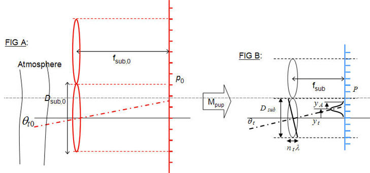
Figure B shows the physical WFS lenslets, whose parameters are Dsub, fsub. In the focal plane of the lenslets, we have a sensor pixel width p, where p is one pixel of a 2D array sensor. (In the physical system, there will probably be a subsequent reimaging of the p focal plane, in order to create a desired p value from a given array sensor whose physical pixel pitch is actually some other value p'; see Figure (MC1) in the later discussion for a concrete example). The equivalent lenslet system (Figure A) lies in the entrance-pupil plane of the actual optical system. The transverse magnification from A to B is the pupil magnification Mpup, a design parameter of the actual optical system. The parameters of the equivalent WFS system are indicated by "0" subscripts.
It is clear that Dsub should scale according to
Dsub,0 = Dsub / Mpup. (Eq. 1)
In the Figure A-B mapping diagram, we also assume that p scales according to
p0 = p / Mpup . (Eq. 2)
(Equation 2 is a modeling choice, not a requirement. A different choice could be made, but Eq. 2 is the simplest choice; furthermore, there is no loss of generality because of this choice).
Now as discussed above, a key constraint that we must observe in order to create a faithful object-space model is the correct mapping of the angle subtended by a sensor pixel (or more precisely, any field angle). In the physical WFS, we have by definition θsnspix = p / fsub ; similarly,
in the equivalent entrance-pupil system, we have θsnspix,0 = p0 / fsub,0 .
On the other hand, from first-order optics, we know that any field angle (or we can think in terms of a system chief ray) must map according to
θsnspix,0 = θsnspix * Mpup (Eq. 3)
Combining the last three formulas, we see that they require
fsub,0 = fsub / (Mpup)2 (Eq. 4)
In sum, we can create a consistent entrance-pupil model of the Shack-Hartmann WFS, as diagrammed in Figures A-B, if we satisfy the 4 conditions of Eq. (1-4). The first three may be consider "obvious" properties of transverse magnification, but the longitudinal magnification required by Eq. (4) is less obvious.
Defining the entrance-pupil system without a physical-system design:
In many simulation exercises, the physical dimensions
{Dsub, fsub, p, Mpup} (Spec "S1.1")
may not be known, because there is no actual optical system design yet. In such cases, which are typical of generic AO system modeling, there are various combinations that one could use to define the WFS system. One option is to specify the set
{Dsub,0 , θsnspix,0 , p0} (Spec "S1.2")
as the fundamental input specifications, with only the picture of Figure (A) in mind.
Note 1: instead of p0 directly in "S1.2", the most meaningful spec may be the "number of sensor pixels per subaperture", i.e., the ratio Npix_per_sub = Dsub,0 / p0 .
Note 2: the Dsub,0 value would generally chosen on the basis of an expected atmospheric Fried-r0 value.
Note 3: θsnspix,0 is independent of Dsub,0 , but there is the following constraint. Since the subaperture diffraction lobe width is l / Dsub,0 , one wants to select values of θsnspix,0 that allow reasonable sensitivity to at least a wave or more of tilt-induced spot motion.
Note 4: One wave of tilt across the full subaperture corresponds exactly to a spot-center angle displacement of l/ Dsub,0 . Note that the boundary of the subaperture occurs at an angle equal to
(0.5*Dsub,0 / fsub,0) = (0.5*Dsub,0) * θsnspix,0 / p0.
The set "S1.2" in conjunction with Figure (A) is a complete and consistent specification, as proven by the preceding analysis. However, the HartmannWfsDft module requires a focalLength specification, and this must be simply fsub,0 = p0 / qsnspix,0.
Summary of HartmannWfsDft parameters thus far:
The preceding analysis has explained how to set the HartmannWfsDft parameters subapWidth andfocalDistance. Usually, we also set detectorPlaneDistance = focalDistance. If one wants to study the effects of defocus on the WFS operation, one can set detectorPlaneDistance to a value of interest different from focalDistance.
Next, we discuss the HartmannWfsDft parameters dxyDetector, overlapRatio, and nxyDetector.
Fourier transform propagation control parameters in HartmannWfsDft
The parameters dxyDetector and overlapRatio control the numerical propagation mesh used by the Discrete Fourier Transform (DFT), when a given subaperture spot diffraction pattern is computed. Given the complex optical field incident on its lenslet plane (see Figure A). HartmannWfsDft first extracts that portion of the field incident on a given subapWidth, interpolates the incident field onto a desired (usually finer) mesh, pads that with a certain band of zeros, and finally performs a DFT to obtain the sensor-plane spot intensity pattern for the given subaperture. This operation is performed separately for each subaperture.
The two parameters dxyDetector and overlapRatio determine the DFT numerical mesh as follows. First, dxyDetector specifies the spacing of the mesh on which HartmannWfsDft will report itsintegrated_intensity output map. The numerical value dxyDetector should be selected so that the diffraction-limited spot is reasonably well sampled: this means at least two samples per(wavelength/subapWidth)*focalDistance.
The more mysterious parameter is overlapRatio: this specifies the total width of the computational mesh for a single subaperture spot pattern. Physically, diffraction causes the spot pattern to have unlimited width; for numerical computation one must decide where to cut this off. overlapRatio specifies the cutoff in terms of thesubapWidth, as follows: overlapRatio = 0 means that the mesh on which the spot pattern is computed in the sensor plane spans exactly one subapWidth; overlapRatio = 1 means that the mesh spans out to one subaperture width on each side of the saubaperture in question, etc; fractional values are allowed. IfoverlapRatio > 0 is specified, HartmannWfsDft will eventually add the overlapping intensity contributions in order to produce its net integrated_intensity sensor-plane output map.
(For a fixed dxyDetector, larger values of overlapRatio of course require longer numerical computation times. Given that some thresholding is usually applied later when computing the spot centroids, overlapRatio= 0 is often satisfactory).
Finally, parameter nxyDetector specifies the total width of the mesh (in number of mesh points) on which HartmannWfsDft produces the net integrated_intensity output map. This should be specified large enough to contain all the subapertures in the 2D layout. A typical setting would be
nxyDetector = (Dsub,0 / dxyDetector) * Nmax,sub + 1 ,
where Nmax,sub is the number of subapertures across the maximal dimension of the 2D layout.
Remaining parameters of HartmannWfsDft
To complete the discussion of Approach 1 to setting WFS parameters, we now explain the remaining parameters.
magnification: In approach 1, the magnification parameter should be set to 1. This means it will have no effect on the computations. This modeling parameter is NOT the pupil magnification Mpup that played a prominent role in Figures A-B and the related discussion. magnification is only needed if we use Approach 2 to defining WFS parameters.
dxyPupil, nxyPupil: These parameters are only used if the "wavesharing" feature is invoked in LightLike propagations. "Wavesharing" is an advanced, not fully-debugged feature of LightLike. For most LightLike use, dxyPupil and nxyPupil should be set to dxyprop and nxyprop, respectively. (Unless "wavesharing" is invoked, the numerical values are actually never used).
xslope0, yslope0: These are the initial values of the slopes, prior to any sensor information being generated in the LightLike simulation. The values are usually set to 0.0.
slopes output: high-resolution and recomputed slopes
Having completed the discussion of Approach 1 to setting WFS parameters, we pause for a moment to discuss some features of the HartmannWfsDft outputs. After that, we return to the alternate approaches to specifying the WFS parameters.
integrated_intensity: this is a composite integrated-intensity map of all the subaperture spots, at all the specified sensor output times. It is recorded on the spatial mesh {dxyDetector, nxyDetector}.
slopes: this is a composite vector containing, first, the x-slopes (tilts) in each subaperture, followed by the y-slopes in each subaperture. The slopes are in units of radians. The order of subapertures within the vector is explained in detail in the Adaptive Optics Configuration Guide.
Each slope is determined from the centroid of the respective subaperture intensity pattern, as recorded on the dxyDetector mesh, with a 10% threshold applied before computing the centroid. The threshold is applied separately in each subaperture processing region. We refer to these slopes as the "high-resolution" slopes.
The "high-resolution" slopes generated as discussed above are intended to be an idealized computation of the subaperture tilts. To more accurately model the centroids computed from an actual 2D array sensor placed in the lenslet focal plane, one should add the LightLike components SensorNoise and HartmannWfsProcessing.
SensorNoise would take as an input the integrated_intensity output of HartmannWfsDft. SensorNoise serves two functions:
(i) SensorNoise allows the spatial integration of the high-resolution integrated_intensity pattern into physical-pixel powers. The "physical pixel" width is the p0 parameter discussed earlier. Note that we used a mental picture of the desired p0 while defining the HartmannWfsDft parameters, but the sample mesh in the sensor plane was actually the finer dxyDetector.
(ii) SensorNoise allows the inclusion of various kinds of sensing noise.
Finally, HartmannWfsProcessing can take as input the physical-pixel powers (more precisely, the discretized "detector counts") output of SensorNoise, and perform new centroid (and slopes) calculations. The latter slopes will include the discretization errors that result from applying a centroid algorithm to the measurement results from the physical sensor pixels.
WFS modeling - details of "Approach 2" (using magnification ≠ 1)
Approach 1 made a simple and physically clear modeling choice about the {p , p0} transverse scaling. In that approach, p/p0 is exactly the same as the pupil magnfication Dsub/Dsub0. The pictorial representation of the model is Figure A-B. As a consequence, we saw that the longitudinal ratio fsub / fsub,0 had to scale as the square of the pupil magnification. In Approach 1, The HartmannWfsDft parameter called magnification, which is NOT the pupil magnification, is set to 1 (i.e., the parameter is inactive).
A different approach is also possible. This alternate "Approach 2" has been used in a variety of LightLike applications, including the important example system BLAT. Approach 2 is somewhat more convoluted, and requires a peculiar "magnification" operation that is implemented by the HartmannWfsDft parameter called magnification.
Approach 2 is based on setting fsub,0 (focalDistance) equal to the arbitrary reference value 1 m. The motivation for the choice focalDistance = 1 was briefly reviewed in the introductory section on WFS modeling in object space. After this choice, Approach 2 completes the specifications by also choosing Dsub,0 and θsnspix,0 . A consistent model can be built on this basis, but it requires an extra adjustment. The problem is that the combination {fsub,0 = 1m, qsnspix,0 } contradicts the intuitive scaling choice p/p0 = Dsub/Dsub0. As we noted before, this is not wrong, but it requires an extra adjustment to the center-center separations of the subaperture regions in the sensor plane. This adjustment factor is what is generated by setting magnification≠ 1. For an example of the actual setting expression assignments, we refer the user to the LightLike distribution's BLAT example system.
As a final comment on the use of magnification ≠ 1, we note the following peculiar property. The diffraction lobe of a subaperture has the width
(wavelength/subapWidth) * focalDistance = (wavelength/subapWidth) * (1m), unaffected bymagnification , but the center-center separation of the neighboring subaperture diffraction patterns is the subaperture separation multiplied by magnification.
WFS modeling - "Approach 3"
In all of the above, we assumed that an adequate simulation model could be constructed without explicitly modeling the physical propagation through the optical train. (Or said more precisely, we assumed that an adequate simulation model could be constructed using just a single physical propagation from the equivalent lenslet plane to the equivalent focal plane.) This is certainly true in many cases. On the other hand, for a faithful model of certain complex systems, it may be necessary to model engineering details of the system by explicitly including beam compression stages and physical propagations between optical components. LightLike has components in the general distribution that allow this extra level of detail, if users feel that is necessary for their modeling purposes.
Miscellaneous comments
Lenslet Fresnel number in Approach 1:
Since Mpup = Dsub / Dsub,0 , Equation (4) is equivalent to the statement
(Dsub,0)2 / (λ fsub,0) = (Dsub)2 / (λ fsub) ,
in other words, Equation (4) is equivalent to saying that fsub,0 must be chosen to conserve the Fresnel number of the lenslet system.
Explicit design of the reimaging stages:
For more complete visualization of the WFS parameter setting procedures, it may be helpful to consider a more complete optical design from primary aperture to physical WFS. Figure (MC1) shows such a layout.
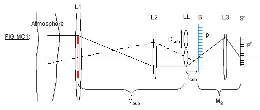
The first key operation in Figure (MC1) is reimaging of the primary aperture L1 onto the actual WFS lenslet plane LL. This occurs with a transverse magnification Mpup. Figure (MC1) shows this reimaging operation being done by a single focusing element L2. In general, the operation may be accomplished by multiple pupil relays, but it is always characterized by an overall Mpup. The red lenslet in the L1 plane is the geometrical back-image of a physical lenslet. In the focal plane S of the physical lenslets, we have the initial focal spots formed by the lenslets. In order to mate available lenslet hardware with available 2D-array sensor hardware, there may be a reimaging of the focal spots, as indicated by the MS magnification operation performed by L3. The symbol p' denotes the actual pixel width on the physical 2D-sensor plane, whereas p denotes the back-imaged size of the sensor pixels in the original lenslet focal plane S.
Concluding remarks
In the present section, we have reviewed procedures for setting the key scalar parameters in HartmannWfsDft. As noted previously, in order to complete the specification of the 2D layout of the WFS subapertures, use of theAOGeom tool is also required. The Adaptive Optics Configuration Guide explains how to use this tool to create subaperture 2D-layout data for input into the HartmannWfsDft parameters xSubap and ySubap.
Remember also that the example system and tutorial information for the BLAT model.provides a working LightLike AO system, which users can consult for further guidance or modify as they wish for their own purposes.
Deformable Mirror

To use the information from a wavefront sensor to produce real-time correction of a wavefront, we require a deformable mirror (DM). The figure at right shows the interface of LightLike's DeformableMirror component. DeformableMirrorapplies specified mirror actuator commands to generate a shape deformation that corrects the wavefront incident on the DM. The commands fed to DeformableMirror must be generated by first multiplying the composite vector of Shack-Hartmann tilts by a "reconstructor" matrix. Then, one would apply a Gain factor and generate the new actuator commands for input to DeformableMirror.
As was the case with the WFS, use of DeformableMirror in a LightLike system requires a preliminary setup procedure. In this setup procedure, we must
(i) specify certain geometric parameters of the DM actuator layout,
(ii) specify a DM influence function, and
(iii) generate.a reconstructor matrix (which will map measured WFS slopes into a mirror shape correction.
The procedure starts by using the same AOGeom helper program (MATLAB-based) that was used to define the 2D WFS layout. Then, a variety of associated MATLAB tools and routines can be used to generate the reconstructor matrix.
A separate Adaptive Optics Configuration Guide is provided to explain the details of the AOGeom and associated LightLike tools. We recommend that the user first study the present section of the general User Guide, and then dive into the Adaptive Optics Configuration Guide.
Finally, remember that the example system and tutorial information for the BLAT model provides a working LightLike AO system, which users can consult for further guidance or modify as they wish for their own purposes. BLAT may help users to get started without diving into all the details of the Adaptive Optics Configuration Guide.
Tilt tracker
In addition to a WFS and DM, many AO systems contain a tilt-tracker subsystem. The purpose of the tilt tracker is to
(i) sense the average tilt of the wavefront, and then
(ii) compensate that tilt before presenting the residual perturbed wavefront to the WFS-DM subsystem.
This typically allows the DM to operate with reduced actuator-stroke requirements. In some cases, a tilt-tracker alone may comprise the complete AO system.
The key new component that we need to perform tilt tracking in LightLike is 
BeamSteeringMirror. The figure at right shows the interface of LightLike's BeamSteeringMirror component.
An average tilt can be sensed in various ways. The most basic would be to split off a portion of the wavefront into a Camera component, and then compute the centroid of the image (or some other measure of image "center"). Centroids can be computed, for example, by using the FpaProcessing module. Given the centroid angular position, one would apply a desired Gain factor and then generate a new tilt command for input to the BeamSteeringMirror module. The BeamSteeringMirror module then modifies the tilt of the incident wavefront before the wavefront passes on the WFS-AO subsystem and to system imaging cameras.
The centroid computation is only one way of determining the tilt correction to be applied. More complicated algorithms, such as correlation measures, may be more appropriate for certain situations. Such algorithms are not provided in the general LightLike distribution, and must be custom-coded. In all cases, though, the tilt compensation is carried out by a final tilt command fed to BeamSteeringMirror.
Again, the example system and tutorial information for the BLAT model provides a working LightLike AO system, which includes a centroid-based tilt tracker. Users can consult the BLAT system for further guidance, or modify it as they wish for their own purposes. BLAT may help users to get started without diving into all the setup details from scratch.