Use of the Zernike function orthogonal basis set is common in optical analysis. LightLike provides a number of components that facilitate the creation of Zernike superpositions, decompositions and related manipulations. Users should exercise caution in two respects when using these components:
(a) The LightLike components offer various normalization and index ordering conventions (reflecting various usages in the general literature on Zernikes).
(b) Zernikes as a mathematical basis set can of course be used to expand a function f(x,y) of arbitrary physical units and significance. However, the most common application is to expand a phase or OPD map, which is (or will later be) associated with an optical phasor exp[i*f(x,y)]. In such cases, it is usually important to be aware of whether the optical path length or difference (OPL or OPD) is expected or provided in meters or in radians of phase.
In this section, we identify and discuss several of the key Zernike components, and we explain the index ordering, normalization and physical units conventions.
Basic Zernike Components
Browsing the ProcessingLib reveals a variety of components related to Zernike manipulations. The two basic operations are:
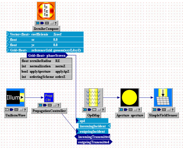
(1) To create a map f(xi,yj) = Sk ak*Zk(xi,yj) , from coefficients ak and Zernike basis functions Zk, i.e., to create a superposition of Zernike basis functions, use the component ZernikeCompose.
Key inputs and parameters are the coefficient vector, ak, and the (x,y) mesh specification. The output is a Grid<double> variable that contains the f(xi,yj) data. Notice that ZernikeCompose does not directly create a LightLike (i.e., a complex field) as output. Typically (but not always), one would want to insert f(xi,yj) as the phase map of a wave at some point in a LightLike propagation system. The picture below shows a simple example, wherein Zernike phase aberrations are added to a plane wave:
(2) To decompose a given function map f(xi,yj) into its ak Zernike coefficients, use the component ZernikeDecompose.
This function is the inverse of ZernikeCompose. Notice that ZernikeDecompose does not accept a Light (i.e., a complex field) as input: the input is simply the real function f(xi,yj) that is to be decomposed.
Ordering conventions
LightLike's Zernike ordering and normalization options are described rather confusedly in the html help pages of the individual components. In the following two subsections, we attempt to clarify the key points.
Each Zernike basis function is a product of a radial and an angular function. As with other orthogonal expansions in 2D, the "natural" indexing to specify a particular basis function uses two indices. However, R.J. Noll wrote an influential paper applying Zernikes to atmospheric turbulence, and in this paper Noll introduced a mapping to a one-dimensional Zernike index. This type of 1D index is used to specify the input or output coefficient vectors, ak, in the Zernike components. A variation (still 1D) of the Noll ordering, used by Malacara, is also available in the LightLike components. Malacara's ordering differs from Noll's in the order of the azimuthal terms within each radial order.
Note that in the i/o of the basic routines, the
ZernikeCompose input vector "coefficients"
ZernikeDecompose output vector "ZernikeCoefs"
are ordered in the 1D convention of Noll or Malacara. Noll order is specified by setting parameter "orderingScheme"=1, and Malacara order is specified by setting "orderingScheme"=2.
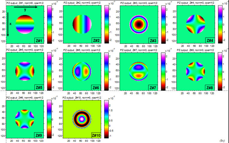
The piston term (constant with respect to x,y) is omitted from all the basic LightLike Zernike components. The coefficients vectors start with tilt. The following picture shows image plots of LightLike's first 10 Zernike functions (Z1 to Z10) in the Noll ordering convention. Note that +x is vertically down in each subplot. Terms 1 and 2 are tilt, term 3 is quadratic focus, terms 4 and 5 are astigmatism, terms 6 and 7 are coma, terms 8 and 9 are triangular astigmatism, and term 10 is balanced spherical aberration and focus:
1) Noll, Robert J., "Zernike Polynomials and Atmospheric Turbulence", J. Opt. Soc. Am., Vol. 66, No. 3, pp. 207-211, 1976.
2) Malacara, D., and S.L. DeVore, "Interferogram evaluation and wavefront fitting": pg. 465, Ch. 13 of Optical Shop Testing, 2nd. ed., D. Malacara, ed., Wiley, 1992.
Normalization conventions
Several normalization conventions for the Zernikes may be found in the optical literature. The LightLike components all have a choice of normalization conventions, specified by the parameter "normalization". Two of the LightLike normalization choices are useful:
"normalization" = 0: The numerical value of each Zk(x,y) peaks at +1 at one or more points on the circle whose radius is the "Zernike radius".
"normalization" = 3: The rms deviation of each Zk(x,y), over the disk whose radius is the "Zernike radius", is equal to 1. Therefore, the numerical coefficient value ak will be the rms value of the product ak*Zk(x,y). Furthermore, in a sum of several terms, .f(xi,yj) = S(k=1,N) ak*Zk(xi,yj), the spatial variance of f will be the sum of the variances of the individual terms, i.e., var(f) = a12+...+aN2 . (This norm is called the "Noll/Malacara norm" in the component help pages).
Other values of "normalization" (which are described in the help pages for individual Zernike components) remain in the routines for historical reasons, but are not recommended.
The "Zernike radius"
The main significance of the "zernikeRadius" parameter has already been indicated in the preceding subsection on normalization conventions. In ZernikeCompose, the extra parameter "applyAperture" allows the generated Zernike terms to be set to zero or not, as desired, for (x,y) coordinates outside the "zernikeRadius".
Physical units
The mesh coordinates (xi,yj) and the Zernike radius, as with all lengths in LightLike, must be specified in meters. The Zk quantities themselves are unitless. Finally, the units in which ak, and thus f(xi,yj) = Skak*Zk(xi,yj), should be specified depend on how f(xi,yj) will be used by LightLike. A typical LightLike procedure would be to input f(xi,yj) into an OpdMap module, in order to apply f(xi,yj) as a phase perturbation on a passing wave (see the picture in Basic Zernike Components). In this case, since OPDmap interprets its input as an OPD in meters, the ak coefficients must be provided in meters. But of course a Zernike sum f(xi,yj) could be used in other ways, where f has different physical significance and different units..
Other Zernike components
The ZernikeCompose/ZernikeDecompose routines explained in Basic Zernike Components should be considered the first choices in LightLike system construction requiring Zernike manipulations. However, in the course of LightLike development and application, a slightly different set of Zernike-related routines was also created. This alternate set of routines shares some but not all features and conventions ofZernikeCompose/ZernikeDecompose.
The "PhaseZernikeXXX" component group:
The component PhaseZernikeOPD is conceptually equivalent to ZernikeCompose. That is, its principal purpose is to accept a set of input coefficients, and then output the sum f(xi,yj) = Sk ak*Zk(xi,yj), on a specified(xi,yj) mesh. The principal differences are:
(i) To produce an output f in meters, PhaseZernikeOPD requires input coefficients in radians of phase at a specified reference wavelength. The output, in meters, is then appropriate for input into the OpdMap module, exactly as was done in the ZernikeCompose illustration in Basic Zernike Components.
(ii) PhaseZernikeOPD requests a Zernike diameter (which is simply called "aperture diameter"), whereas ZernikeCompose requests a Zernike radius.
(iii) PhaseZernikeOPD has parameters named "m_vec" and "l_vec" that allow extra selection freedom by specifying that only certain subsets of the input coefficient vector elements be used when composing the Zernike sum.
In other respects, the ordering and normalization convention options for the coefficient input vector are identical inPhaseZernikeOPD and ZernikeCompose .
There are several other special-purpose Zernike-related components whose i/o conventions matchPhaseZernikeOPD. The most important are PhaseZernikeDM, and PhaseZernikeSlopes:
PhaseZernikeDM takes an input vector of Zernike coefficients, internally composes the sum function f, and generates corresponding deformable-mirror (DM) commands which are organized as required for input into the LightLike DM component.
PhaseZernikeSlopes takes an input vector of Zernike coefficients, internally composes the sum function f, and generates the corresponding wavefront-sensor (WFS) slopes, corresponding to Shack-Hartmann subapertures whose geometry is specified according to the LightLike WFS procedures.