This task differs from the underlying reconstruction of a wavefront in two ways:
(1) we have the extra complication of DM facesheet influence functions;
(2) in closed-loop operation with a DM, the WFS slopes represent the difference ("error") between the mirror shape and the wavefront. We now want to develop a reconstructor mapping that directly converts sdata into the actuator displacements δdact required to null the residual WF perturbation: δdact,rec = R sdata . For closed-loop operation with a DM, we use the notation δd to emphasize the fact that, at any time instant, the WFS slopes represent the difference between the mirror shape and the wavefront, so that δdact,rec represents the change that needs to made to the current actuator displacements. The new commands to be specified to the mirror would be dact,new = dact,old +δdact,rec.
Deformable mirror influence functions (OPD and slope)
A continuous DM facesheet has some stiffness, so that pushing or pulling the facesheet with a point-like actuator tip may cause facesheet displacement at significant distance from that actuator, with a particular deformation shape. Provided that the mirror is operating in a regime where the superposition principle applies, the net deformation can be expressed as the sum of the deformations due to the individual actuators. The deformations at a set of discrete points can then be expressed in terms of the actuator displacements by means of a matrix multiplication. In the AO tools, this matrix is called the "OPD influence function", although we should bear in mind that the matrix yields thesurface displacements.
We use the notation
dact = vector of actuator displacements, dim (nact x 1), in units of m
dsrf = vector of mirror surface displacements, dim (nopd x 1), in units of m.
We express the dimension of dsrf as nopd because at each surface point we
can compute the resulting opd correction to the incident wavefront. The AO
tools allow this opd mesh to be specified with a density higher than the actuator
or subaperture mesh.
The DM OPD influence matrix is defined by the relation
dsrf = Adact , where the OPD influence matrix, A, has dims (nopd x nact).
Depending on how well one wishes to resolve the DM surface shape,
the dimension nopd may be very large. However, the number of surface
elements affected by a given actuator is usually small compared to nopd.
That is, most elements of A are 0, and A can be stored in a sparse format.
When the DM is used at near-normal incidence (the usual practice), the DM surface deformation produces an opd change in the (already perturbed) incident wavefront of
δdopd = 2dsrf = 2Adact .
Now, in closed-loop operation, the WFS slopes represent the difference between the current mirror shape and the wavefront. If we denote this difference as δdopd, then we can write
s = S' δdopd , where matrix S' has dims (2nsub x nopd).
The matrix S' could be taken as the S'c matrix that we defined for zonal wavefront reconstruction, ifwe define the opd mesh to be exactly the actuator mesh. However, for generality, we allow the opd mesh to be denser. Combining the previous equations yields
s = 2S'A δdact
= S δdact , where matrix S has dims (2nsub x nact), and where δdact denotes the
extra actuator displacements required to null the current slopes.
Any matrix S that takes actuator displacements into slopes is called a DM slope influence matrix.
The AO tools function aoinf computes linked DM opd and slope influence matrices. A complication that arises in practical DM systems is that we do not necessarily treat all actuators on an equal footing. As discussed in connection with aogeom, we may classify actuators as either masters or slaves. In that case, the DM slope influence matrix, S, must be further refined. The aoinf function includes this refinement if the geometry setup has specified a non-zero number of slaves. The zonal reconstructor discussed next allows for this refinement. Note that the master-slave distinction has no impact on the DM opd influence function, A: the A matrix operates on all the actuators, and has the same values regardless of slaving identifications.
Choice of influence function shape
The values of the A matrix computed by aoinf depend on the specification of an analytic model for the facesheet deformation due to a point force. The LightLike AO tools provide five choices of influence function shape for the OPD influence function. Since the shape is considered geometry information, the specification of shape is done in the aogeom GUI. The shape choices are denoted as Green's Function, Gaussian, Piston, Linear, and Cubic. For a given shape category, the user also specifies width parameters. Details are given in the AO Geometry Parameters section, in the subsection Influence Function Entries. Given a choice of shape and width parameters, the subsequent execution of aoinf generates the corresponding DM OPD and slope influence matrices.
Zonal reconstructor for DM actuator commands
To obtain DM actuator commands using a zonal reconstruction, we will require the AO tools functions aogeom, aoinf, and aorecon. aogeom is used to establish the geometry of subapertures and their corner actuator positions, as introduced previously.
In the previous section on DM influence functions, we obtained a matrix S defined by
s = S δdact , where matrix S has dims (2nsub x nact).
Given S and some WFS data sdata, we must solve the preceding equation for the δdact to find the additional mirror deformation required to null the current error. The solution requires a least-squares or "pseudo-inversion" approach, since S has more rows than columns. Using the superscript notation (...)# to indicate a pseudo-inverse operation, we write formally
δdact = S# sdata = Rzon sdata ,
defining the zonal reconstructor matrix Rzon = S#. The AO tools function aorecon is provided to compute the pseudo-inverse of any specified matrix. Details of the available options, and examples of Matlab terminal sessions, are given in the later section devoted to aorecon. One of the key options of aorecon is the capability to perform singular value decomposition.
Refinement of the influence function: master and slave actuators, and actuator voltages
The above paragraphs define the zonal reconstruction concept, but when using the AO tools functions the user must be aware of several complications and refinements. These refinements do not require extra steps on the user's part, but they introduce extra terminology and variables which may initially cause some confusion. In future releases, we plan to clean up and streamline the present procedure.
Frequently, the actuators of a DM are not all treated on equal footing, in the following sense. As discussed in further detail in the geometry section, active (i.e., non-inert) actuators are divided into the categories of "masters" and "slaves". The displacement of a slave actuator is constrained to be a fixed linear combination of a few neighboring master displacements. If we have slaves in the DM configuration, then in order to guarantee the desired slaving relations, the slope influence function should be modified to automatically incorporate the slaving constraints. The result is a modified influence function that maps a vector of only master actuators to all the subaperture slopes. This modified influence function, rather than the full S, is the quantity that will be pseudo-inverted to form the reconstructor.
A final complication that is allowed for by the AO tools concerns a conversion between actuator displacements and actuator voltages. The voltages are the physical input quantities provided to a DM by a physical hardware control loop. The motivation for modeling this extra degree of freedom was not to represent a simple proportionality factor between applied voltage and displacement. The original motivation was to model cross-talk that existed with a specific DM that was of interest during early stages of LightLike development. The original motivation is no longer relevant, and in contemporary work with LightLike, the voltage-to-actuator displacement matrix is by default the diagonal unit matrix. The only reason for discussing this here is that, when working with some of the AO tools functions, the user must deal with variable names that reflect this early side-track in development.
The refinements discussed in the preceding two paragraphs are expressed quantitatively by the chain of linear mappings δdact <== δvact <== δvmas , where δdact is the vector of all actuator displacements, δvact is the vector of all actuator voltages, and δvmas is the vector of master actuator voltages. Therefore, the original formulation of the slope influence function, s = S δdact , becomes
s = S δdact
= S * (vtod) * (mvtov) * δvmas
= (mvtos) * δvmas ,
where we have introduced notation of programming-variable style:
(mvtov) = matrix that maps master-actuator volts to all-actuator volts (dims nact x nmas)
(vtod) = matrix that maps all-actuator volts to all-actuator displacements (dims nact x nact)
(mvtos) = matrix that maps master-actuator volts to all subaperture slopes (dims 2nsub x nmas)
The matrix names written in programming style are actual variable names generated in the Matlab workspace when using the AO tools functions. A full list of variable names is given in a later reference section.
The key points for the AO tools user are:
(1) The composite matrix (mvtos) is automatically computed by running the function aoinf. An example of the Matlab command sequence is given in the section where syntax details of aoinf are specified.
(2) The composite matrix (mvtos) is the input variable that must be pseudo-inverted when using the aorecon function to finally compute the reconstructor. This holds even if no slave actuators have been defined in the geometry.
(3) The OPD influence matrix generated by aoinf, denoted A in our theoretical development, has the Matlab variable name (opdif).
In sum, zonal reconstruction of DM actuator commands requires the use of tools functions aogeom(define geometry), aoinf (compute A and mvtos), and aorecon (compute pseudo-inverse of mvtos).
Tilt removal option
In AO systems that contain both a fast-steering mirror and a WFS, some undesirable coupling may occur if both elements are trying to correct residual tilt. Therefore, an important option provided by routine aorecon is the computation of tilt-included or tilt-removed reconstructors. "Tilt-included" signifies that the reconstructor will generate an estimate of the complete wavefront impinging on the WFS, whereas "tilt-removed" signifies that the full-aperture tilt term is projected out of the reconstructed wavefront. The tilt-removal option is independent of the SVD option.
Waffle-mode removal option
The Fried geometry of subaperture-actuator placement is susceptible to the appearance of a particular unsensed DM mode called "waffle". This consists of a saddle-like deformation of the surface patch corresponding to any subaperture, where the two actuators on one diagonal are equally high, and the two actuators on the other diagonal are equally low. The pattern is illustrated in Figure 6 over a neighborhood of 3 x 3 subapertures. Due to the symmetry, this produces WFS focal-plane spots whose centroid is undisturbed relative to the spots of a flat wavefront: hence, we have an "unsensed mode". Higher moments of the spot shape are affected, but the centroid is not sensitive to those moments.
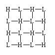
Figure 6: "Waffle" surface deformation in the Fried geometry. H and L mark actuator locations, where H represents a high actuator and L represents a low actuator. The squares define the subaperture areas.
The LightLike AO tools offer a reconstructor option that attempts to explicitly remove the waffle component from the actuator command vector. The so-called waffle-constrained reconstructor is a zonal reconstruction method for actuator commands that uses the sequence of AO tools functions aogeom (define geometry), lsfptosw (compute a slope and waffle influence matrix), and aorecon(compute pseudo-inverse). As its name implies, lsfptosw computes a slope influence matrix using the same meshes and a procedure closely related to the previously discussed lsfptos method. Subsequently, the aorecon function is used in the same way(s) as in previously discussed zonal reconstructions. The function details section includes a sample Matlab terminal session that illustrates a reconstructor calculation using lsfptosw.
Depending on the problem details, the explicit removal of waffle implemented via lsfptosw may be redundant. The use of the SVD capability of aorecon may be sufficient to remove any significant waffle component. Nevertheless, the lsfptosw option is provided in the AO tools, so users may experiment on their own particular problems.
REFERENCES:
Modal reconstructor for DM actuator commands
To obtain DM actuator commands using a modal reconstruction, we will require the AO tools functions aogeom, slope2mod, mod2opd, aoinf, and aorecon. As usual, we start with aogeom to define the geometry of the subapertures.
In the section on modal reconstruction of wavefronts without a DM, we developed the reconstructor
dopd, rec = Z amod, rec = Z V sdata .
As discussed previously, the tools functions slope2mod and mod2opd are used to compute V and Z. Now, in closed loop operation with a DM, the WFS slopes represent the difference between the current mirror shape and the wavefront. If we denote this difference as δdopd, then we can write
δdopd, rec = Z V sdata .
Without a DM, the ZV product gave the final WF reconstructor. But, to drive the DM, we must compute the corresponding actuator displacements. In terms of the DM opd influence matrix, we have
δdopd = 2A δdact , where A has dims (nopd x nact), and the opd mesh must of course be whatever was used to compute Z and V.
As noted previously, the tools function aoinf computes (among other things) the matrix A.
Now, given A, we must solve the preceding equation for the δdact. To do so requires a least-squares or "pseudo-inversion" approach, since A has more rows than columns. Using the superscript notation (...)# to indicate a pseudo-inverse operation, we write formally
δdact,rec = (1/2)A# δdopd = (1/2)A# Z V sdata= Rmod sdata ,
where Rmod = (1/2)A# Z V defines the final modal reconstructor matrix, for reconstruction of the DM actuator commands from the WFS slopes.
The AO tools function aorecon is provided to compute the pseudo-inverse of any specified matrix. Details of the available options, and examples of Matlab terminal sessions, are given in the later section devoted to aorecon. One of the key options of aorecon is the capability to perform singular value decomposition.
In sum, modal reconstruction of DM actuator commands requires the use of tools functions aogeom(define geometry), slope2mod (compute V), mod2opd (compute Z), aoinf (compute A), andaorecon (compute pseudo-inverse A#).