(NOTE: This document is an extract from a longer report. Section numbering in the present extract starts with 4.0)
4.0 Thermal Blooming Usage
Two examples of the use of the thermal blooming code are presented in this section. The first is a simple propagation to the far-field of a Gaussian HEL beam. It duplicates in LightLike a simple configuration created by Lincoln Laboratory and simulated using their MOLLY code. The second uses the phase screens created by a Gaussian HEL to distort light back-propagated from an incoherently illuminated disk. This duplicates an effort of Nahrstedt (Refs.[5]) to study the thermal effects on a back-propagated beam.
4.1 Discussion and Features
The first consideration that needs to be addressed in the configuration of a thermal blooming model is the placement of the phase screens. The LightLike implementation does not provide the user with any guidance for determining the placement or number of thermal screens required to accurately model a given propagation path. We suggest that users experiment with varying the number of screens and their placement along the path to determine what constitutes a “good” approximation for their configuration.
Because the thermal blooming algorithm uses the two-cycle scheme described in section 2.0, there are some constraints imposed by the implemented algorithm on the placement of the screens. This requirement amounts to this: The screens must be positioned in a fashion in which they are located at the midpoint of segments, which partition the propagation path. For example, if we have a 100 km path and place just one phase screen at 90 km; this violates the segment midpoint requirement and so is not a permissible configuration. Using just one phase, one must place it at the midpoint of the path. There is however a way around this requirement. Consider again locating the screen at 90 km, then, if we were to locate a second screen at 40 km, the midpoint requirement would be satisfied. So, do just that but set the absorption coefficient for this screen to be zero. This turns off the thermal blooming and the only thermal effects are those applied by the screen located at 90 km. However, something, which may be undesirable, occurs when the absorption coefficient for the 40 km screen is set to zero; the beam is not attenuated along the first 80 km of the path. This leaves us with the problem: How do we insert the 40 km screen, so as to conform with the requirements of screen positioning, turnoff the thermal blooming effects of this screen, and yet attenuate the beam along the entire path? There is a hack solution to this problem. Set the absorption coefficient to the desired value (probably the same as that of the 90 km screen), and set one of the wind velocity components to a very high number, say 106, or a number, which guarantees that the entire temperature distribution is blown off of the mesh in a time corresponding to the incremental update DeltaTime. This has the effect of applying thermal blooming at the 40 km screen, but the effect of the thermal blooming is negligible since the temperature distribution due to the HEL heating is now off the mesh on which the beam currently lies. Yet, the attenuation specified by the absorption coefficient will still be applied to the beam. As mentioned, this manner of positioning screens satisfies the 2-cycle scheme and conforms to the way in which bookkeeping is currently done in the thermal blooming code.
The use of numberSavedStates is perhaps best illustrated via an example. Consider the somewhat contrived example of an optical path of 1000 km, which gives a propagation time Δ ~ 0.0033 seconds, between source and target. Furthermore, suppose that the update time of a detector in the target plane is Δ/2and the update rate of a detector in the source plane is Let the detector in the target plane request data at time T and the detector in the source plane request data at time, T+3Δ/4 Also, suppose that there are three screen locations: at 250 km, 500 km and at 750 km., as shown in figure 4.1-1. (NOTE: after the rather lengthy discussion concerning the rule regarding the positioning of the thermal screens, this example violates that rule. It is to be regard merely as an illustration of the use of the parameter, numberSavedStates, and these locations serve to simplify the calculations involving time). When the detector in the target plane requests the HEL at time T, the HEL is sent from its source at time T-During its propagation along the optical path the HEL modifies the thermal blooming screens as it encounters them. Figure 4.1. shows the times at which the thermal screens are updated by the HEL and the time at which they are encountered by the back-propagated beam. For instance, the screen in the middle is updated at time T - Δ/2by the HEL created at the source at time T - Δ and at time T by the HEL, which starts out at time T - Δ/2. Now the back-propagated beam BP arrives at the midpoint of the propagation path at time T+Δ/4. This means that the screen updated at time T is the closest, temporally, to the time at which the back-propagated beam arrives at the thermal screen. So it is the first set of thermal saved states that are used in updating the back-propagated beam at time T + Δ/4. On the other hand, at the screen located at 750 km one finds that it is the thermal states corresponding to the time T - Δ/4 that gets used in the application of phase to the back-propagated beam, and these thermal states are saved in the second set of saved states. We find for this configuration at least two past thermal states are needed to correctly update the back-propagated beam, i.e. numberSavedStates must be equal to at least 2.
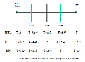
Figure 4.1-1 Shows the locations and corresponding times of various beams.
4.2 Examples
The MOLLY configuration provides an elementary example of thermal blooming. The basic configuration consists of a propagation path of 5000 meters, with a telescope aperture diameter of 0.5 meters. The beam projected to the far-field is a Gaussian beam with a beam sigma (the e-2 point) equal to the radius of the telescope and an initial power of 300000.0 Watts. The wavelength is 3.8e-6 meters. There are 20 thermal screens along the beam path located at the following positions distances = [214.03, 634.885, 1040.07, 1427.165, 1794.0, 2138.75, 2460.0, 2756.805, 3028.725, 3275.8, 3498.525, 3697.8, 3874.845, 4031.265, 4175.445,4318.645, 4464.725, 4613.8, 4765.995,4921.445] in meters. Note the increase in spacing density toward the end of the path. Also, these positions satisfy the midpoint requirement mentioned above. The three physical properties of the screens: absorption coefficient = 6.928e-5 m-1, scatter coefficient = 6.928e-5 m-1,, and temperature = 0.0 C, are the same for each of the screens. There is no beam slewing and the platform and target are stationary. At each of the thermal screens there is a constant wind in the x-direction of 10 m/s. The number of mesh points to sample the beam and the thermal screens is the same, 512X512 and the mesh spacing is 0.1 meters. The incremental update rate is 0.01 seconds. This is also the request rate of the SimpleFieldSensor module in the far-field. This code was run for .11 seconds. It is believed that the MOLLY code uses meshes, which are symmetric about the origin, whereas the LightLike uses asymmetric mesh with the origin at a mesh point. This is probably the source of discrepancy between MOLLY and LightLike.
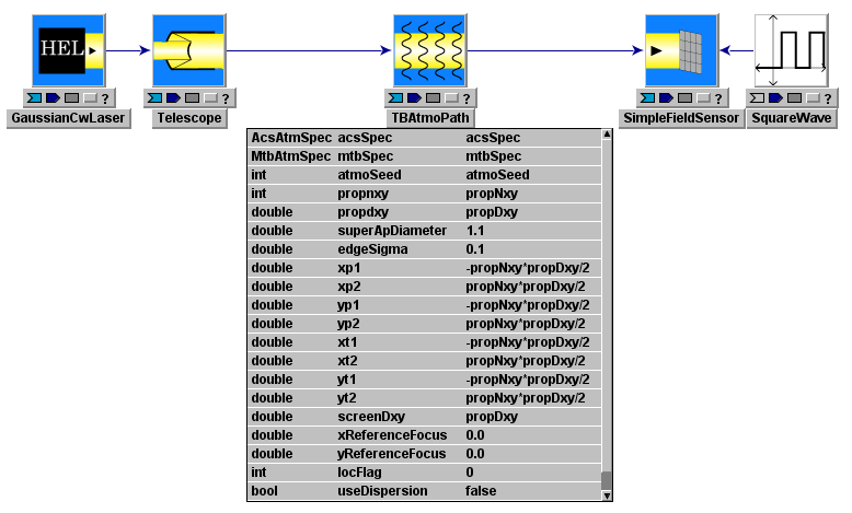
Figure 4.2-1 Top level of the Lincoln Laboratories thermal blooming configuration.
Figure 4.2-1 shows the modules, which comprise the LightLike simulation model. The TBAtmoPath module is shown with its accompanying input parameters. Note the parameters acsSpec and mtbSpec, which provide the information for constructing the phase and thermal blooming screens. MtbAtmSpec(512, 0.1, -1.0, -1.0,.0.01, 6.93e-5,6.820e-5, 0.0, 3.8e-6, distances, 10.0, 0.0, 0.0, 0.0, 0.0, 0.0, 1) and acsSpec is specified simply as AcsAtmSpec(5000.0). Descending into the module TBAtmoPath we see in figure 4.2-2 that it consists of the two PropagationController modules and a TurbBloomAtmosphere module. The information just outlined is also presented in the accompanying runset, shown in figure 4.2-3.

Figure 4.2-2 Descent into TBAtmoPath.
Figure 4.3-3 The Runset specification accompanying the Molly Model
A second example of the thermal blooming code is provided by the configurations outlines in Nahrstedt’s paper [5]. Nahrstedt’s study is designed to investigate the impact of a thermally bloomed atmosphere on a beam back-propagated from the target plane. Configuration specifications outlined in the Nahrstedt study are as follows: the HEL wavelength equals 3.8e-6 meters; the back-propagated beam wavelength equals 10.0e-6 meters; the x-component of the wind speed equals 100 meters per second; the propagation path range equals 107.85 km; the Fresnel number for the configuration is 3.833; the telescope diameter equals 1.0 meters; the absorption number equals 0.274; and the transmission equals 0.760. Additionally, we are told that the HEL is Gaussian (beam waist unknown); that the back-propagated beam is an incoherent uniform disk centered at the point in the target plane at which the intensity of the HEL is maximum, and which subtends an angle of ~10 mirco-radians at the telescope; that the placement of the screens is nearly uniform; and that the geometry for the sampling meshes is a rectangular grid of 64X64 points with a spacing of 0.0476 meters. We modeled the incoherent disk using the IncoherentDisc module with fifteen speckle realization. Five thermal screens were placed uniformly along the path. The simulation was run for six differ distortion numbers [0.333, 0.667, 1.335, 2.670, 5.339, 10.679], where the distortion number was varied by varying the power of the HEL. Here the corresponding power levels are, [0.1, 0.2, 0.4, 0.8, 1.6, 3.2] Mega-Watts. For distortion number Nahrstedt uses
![]()
The factors are P, the HEL power; a, the telescope radius, and R, the propagation path length. The other factors are as defined in section 2.1. In order to generate the thermal screens in LightLike, we need to specify three physical quantities: the absorption coefficient, the scatter coefficient and the temperature. From the data provided, we know that the absorption coefficient is 0.274/107.85e3 m-1, the scatter coefficient is zero, but we need to extract the temperature. Remember in section 3.3 it was shown that tbcoef = -0.2318e-6/273.15+ temperature) = nT/pn0Cp(Note that the factor n0 was taken to be 1.0 in section 2.1). Using this equation and the equation for the distortion number, we find that
![]()
[-2(400000)(0.274/107.85e3)(107.85e3)2/( 100)(.5)3 )][nT/pn0Cp]
which gives that
-0.2318e-6/273.15+ temperature) = nT/pn0Cp=-7.0588e-10, hence the temperature= 55.23C.
For each distortion number, twenty realizations were created and the images in the focal plane of a camera behind the telescope averaged. The update rate was 0.0005 seconds and the stop time 0.015 seconds, for a total of thirty passes through the atmosphere, which guaranteed that a steady-state had been achieved.
5.0 Simulation Results
This section gives a brief comparison of the results obtained by the thermal code in LightLike to those results obtained by the Lincoln Laboratories’ MOLLY code. It also compares results from the Nahrstedt study to those generated with the thermal blooming software in LightLike. These results of course pertain to the systems described in section 4.2 .
5.1 Molly Code Results
Figure 5.1-1 shows a comparison of the far-field intensity footprint of the beam on the eleventh iteration. The image on the left is that obtained by Lincoln Labs and the one on the right the image generated by LightLike. Figures 5.1-2 and 5.1-3 are slices through the peak intensity location of the far-field images, which again compare Lincoln Lab and LightLike results. While the comparisons are reasonably good, there are differences.
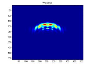
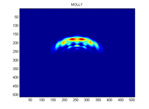
Figure 5.1-1 Far-Field intensity footprints of the thermal bloomed beam. These are steady-state results.
From figures 5.1-2 and 5.1-3 again we see that the slice plot track reasonably well but LightLike produces a greater peak intensity value. Possible reasons for these discrepancies are: there are possibly different filters being applied during the propagation (we are unaware of the details underlying the MOLLY code’s propagator), this could explain the side lobe variation; also, we believe that the MOLLY code’s meshes are symmetric with respect to the origin, while those of LightLike are asymmetric, due to the placing of a mesh point on the origin, which could explain the peak intensity mismatch. Figure 5.1-4 shows a comparison of the time history of the peak intensities from both simulations. As expected the results track well but the LightLike peak intensities are always slightly larger.
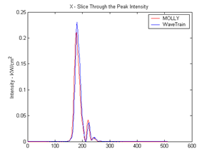
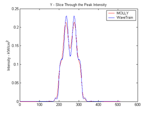
Figure 5.1-2 X-slice and Y-slice plots through the point of peak intensity
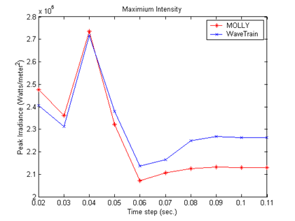
Figure 5.1-3 Comparison of the peak intensity of the far-field versus time.
5.2 Nahrstedt Study Results
Figure 5.2-1 shows the intensity footprint of the forward beam in the far-field for the six different distortion numbers considered in the study. As expected, as the level of thermal blooming is increased the beam defocusing also increases, causing its centroid to move farther off-axis. The results of the principle comparison to the Nahrstedt study are shown in figure 5.2-2. (Relative intensity is the ratio of the peak intensity of the field to the ideal intensity of the field). The curve for the forward beam (HEL) was obtained by computing the relative intensity of the field in the far-field in steady-state. For the back-propagated beam, 20 realizations of the back-propagated beam were computed and the intensities of the beams were averaged. The LightLike results seem to track well with Nahrstedt’s results but do not match exactly. A detailed analysis of the discrepancies is impossible since we do not have the Nahrstedt code. We also had to make guesses about some of the inputs to the simulation, such as the number and locations of the thermal screens, and the nature of the Gaussian beam. Given these uncertainties the discrepancies should be anticipated.
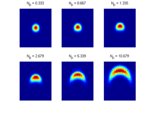
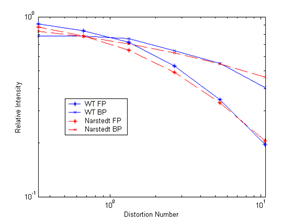
Figure 5.2-1 Intensity footprint of the HEL for six different level of thermal blooming.
Figure 5.2-2 The curves show the relative intensity versus distortion number of the thermal blooming for the six cases mentioned in section 4.1.1. Two sets of curves are shown one for set the forward beam (FP) and one set corresponding to the back-propagated beam (BP).
6.0 REFERENCES
[1]. V.P. Lukin, Atmospheric Adaptive Optics, (translated by P. Schnippnick), SPIE Press, 1995.
[2]. F.G. Gebhardt, “Twenty-Five Years of Thermal Blooming”, SPIE Proceedings Vol. 1221, Propagation of High-Energy Laser Beams Through the Earth’s Atmosphere, pp. 2-25, 1990.
[3]. L.S. Hills, J.E. Long, and F.G. Gebhardt, “Variable Wind Direction Effects on Thermal Blooming Correction”, SPIE Proceedings Vol. 1408, Propagation of High-Energy Laser Beams Through the Earth’s Atmosphere II, pp. 41-53, 1991.
[4]. J.L. Walsh and P.B Ulrich, “Thermal Blooming in the Atmosphere”, J.W. Strohbehn, ed., Laser beam Propagation in Atmosphere, Vol. 25, Topics in Applied Physics, Springer-Verlag, New York, 1978.
[5]. D. Nahrstedt, “Influence of a thermally bloomed atmosphere on target image quality”, Applied Optics, Vol. 21, No. 4, 1982.