The function aorecon computes the pseudo-inverse of a specified matrix, with a variety of options. The matrix to be pseudo-inverted may be generated by aoinf, lsfptos, or some user-supplied analogue. aorecon can compute either tilt-included or tilt-removed reconstructors, and can perform singular value decomposition to suppress near-singular modes. One uses aorecon to carry out different tasks by calling the routine several times, each time with a different argument syntax.
Since aorecon is often the last step in the AO configuration process (see the summary table), it will be convenient to create a save file that contains any reconstructor matrices generated by aoreconplus all the previous variables created by whatever combination of aogeom, lsfptos, aoinf, and other routines was used. Since some of the variables of interest have been saved previously in other files, this creates some redundancy. However, for purposes of later rework or for insertion into a LightLike simulation run, we recommend to collect all relevant variables into one final .mat save file. Because of the number of options available, there is no convenient way for the aorecon function to do this for the user: the user must manually create the save file using Matlab's easy-to-use "save" command. An example is given in one of the following Matlab session examples. To reduce keyboard tedium, the recommended procedure is to save the whole workspace (perhaps after deleting certain temporary work variables that the user has no wish to save).
From the Matlab command line, the possible calling syntaxes for aorecon are:
>> rsv = aorecon(M); % Compute singular values of input matrix
where
M = matrix whose singular values are to be computed
rsv = vector of singular values
OR
>> recon = aorecon(M, ns, tiltopt); % Compute "pseudo-inverse" matrix of M
where
M = matrix whose pseudo-inverse is to be computed
ns = number of singular modes to be removed (may be 0)
tiltopt = 0: compute tilt-included pseudo-inverse
1 or OMITTED: compute tilt-removed pseudo-inverse
recon = pseudo-inverse of input M, subject to ns and tiltopt
UNITS associated with recon are dictated by the input matrix M. That is, if M maps OPD in meters to slope angles in radians of angle, then its pseudo-inverse maps slope angle in radians to OPD in meters.
In the following subsections, we illustrate two applications of aorecon, and we exercise several of the options.
Application to zonal reconstruction of wavefront (no DM)
Here we show how aorecon is used to operate on the output of lsfptos. This produces a zonal reconstruction of a wavefront from slope data, in the absence of a DM. The following sequence of Matlab commands illustrates the procedure. For the origin of the Matlab variables used below, refer to the Matlab excerpt in the section on lsfptos.
% First, we pseudo-invert (including SVD) the S'c slope influence matrix that was computed by lsfptos :
>> rsv = aorecon(ptos); % Calculate the vector of singular values rsv.
The reconstructor WAS NOT computed by this function call.
>> figure; semilogy(rsv,'o-'); % Inspect rsv to determine how many singular values should be suppressed:
% see the graph and discussion below.
>> ns = 2; % From inspection of the plot, it appears we should remove two singular modes.
>> reconti = aorecon(ptos,ns,0); % Compute the tilt-included reconstructor, dim (45x64).
Singular value decomposition: Choosing the number of singular values to remove may not be entirely obvious. The vector rsv usually contains steadily decreasing values which span several orders of magnitude. When there are near-singular modes, there is usually an obvious break point at which the values suddenly drop by several orders of magnitude. The typical result for AO systems appears to be a few near-singular modes which occur towards the end of the vector. In the following plot, we show the singular values of the above ptos matrix. As noted in the Matlab command comments, the plot behavior suggests we should remove two modes:

% We now continue the Matlab example, assuming that the s vector generated in the lsfptos example represents empirical WFS slope data, in radians of angle, from which we will reconstruct the wavefront opd in units of m:
>> opdrec = reconti*s; % Compute vector of reconstructed OPD values, at the "actuator" locations.
% opdrec has dim (nactx1)=(45x1), and units of m.
>> figure; plot(opdrec - opd); % To check the solution, plot the difference between the reconstructed WF and the truth WF, vs. "actuator" index. The plot (not shown here) shows that the difference is tiny, which indicates an accurate reconstruction.
% When working with real WFS data, we often want to make a mesh or image plot of the reconstructed wavefront. The utility function actmap can be used to prepare the OPD vector for this purpose:
>> opdrec2d = actmap(opdrec, xact, yact); % Output opdrec2d is the (nxact x nyact) array that
% rearranges vector opdrec into its 2D layout.
>> figure; imagesc(opdrec2d); axis image; colorbar; xlabel('Y index'); ylabel('X index');
% The resulting image plot is reproduced below. It verifies that the reconstructed WF is a tilted plane with 1 urad of x-tilt, and 2 urad of y-tilt, in agreement with the original WF from which the slope data was constructed (see lsfptos example). In the corners, where there were no "actuators", a default value of OPD equal to the bottom of the color scale was assigned.

Application to zonal reconstruction of DM actuator commands
Here we show how aorecon is used to operate on the output of aoinf. This produces a zonal reconstruction of DM actuator commands from slope data. The following sequence of Matlab commands illustrates the procedure.
>> load small45gi.mat; % Load the output file of aoinf into a clean Matlab workspace.
% (The user need not generate this file: it is provided as an
% example file in the LightLike distribution.)
>> rsv = aorecon(mvtos); % Calculate the vector of singular values rsv.
The reconstructor WAS NOT computed by this function call.
>> figure; semilogy(rsv,'o-'); % Inspect rsv to determine how many singular values should be suppressed:
% see the graph and discussion below.
>> ns=1; % From inspection of the plot, it appears we should remove one singular mode.
>> recon = aorecon(mvtos,ns); % Compute the tilt-removed reconstructor.
>> reconti = aorecon(mvtos,ns,0); % Compute the tilt-included reconstructor.
>> save small45gir.mat % Save the resulting workspace as a *.mat file named "small45gir.mat".
% The file name can be arbitrarily specified by the user.
% NOTE regarding the save file: in contrast to running aoinf, running aorecon does not automatically create a save file. This behavior was chosen because of the number of options that aorecon has. Saving the entire workspace in the above example results in the creation of a single data file with all the data that could be needed by a LightLike simulation run. Of course if the user has created extra working variables in the Matlab session, these may be deleted if desired before saving. However, the presence of extra variables in the save file does no harm. This final save file, which will contain the previously-loaded AO geometry data, the influence function matrices, and one or more reconstructor matrices can be rather large (easily several 10s of MB).
Note that the slope influence-function input to aorecon is the matrix mvtos. As explained in a background section, "volts" are by default equivalent to "displacements" because the current default mapping of actuators volts to displacements (matrix vtod) is the unit matrix.
Singular value decomposition: Choosing the number of singular values to remove may not be entirely obvious. The vector rsv usually contains steadily decreasing values which span several orders of magnitude. But when there are near-singular modes, then there is usually an obvious break point at which the values rapidly decrease by one or two orders of magnitude. The typical result for AO systems appears to be a few near-singular modes which occur towards the end of the vector. In the following plot, the singular values of the influence function in small45gi.mat are plotted:
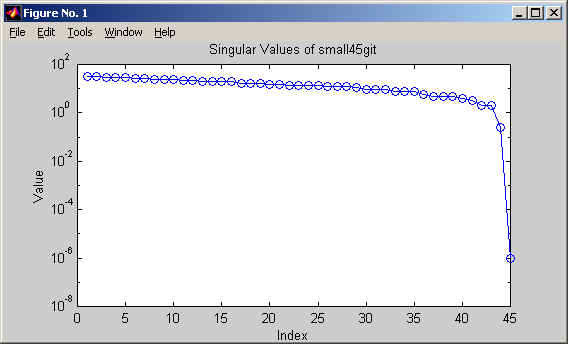
From inspection of the graph, we choose to eliminate 1 singluar mode, because of the drop of more than four orders of magnitude between the 44th and 45th points. One might be tempted to try 2 singular values because of the drop of one order of magnitude between the 43rd and 44th values; but, it has been our experience that one should only suppress the singular values which are roughly of the same order of magnitude as the lowest value.
Variables contained in the output file: As explained at the end of the sample Matlab session, the save file will contain one or more reconstructor matrices, whose names were user-specified, plus all the preceding data created by aogeom and aoinf. The names and format of these variables are defined in the section .mat Interface File Contents.